Numerical computation of the density of states of aperiodic multiscale Schrödinger operators

Cancès, Eric; Massatt, Daniel; Meng, Long; Polack, Étienne; Quan, Xue

doi:10.48550/arXiv.2510.15369

Numerical computation of the density of states of aperiodic multiscale Schrödinger operators

Eric Cancès¹¹1Eric Cancès, CERMICS, École des Ponts, Institut Polytechnique de Paris, and Inria, 6 and 8 av. Pascal, 77455 Marne-la-Vallée, France (eric.cances@enpc.fr) Daniel Massatt²²2Daniel Massatt, New Jersey Institute of Technology, NJ, USA (daniel.massatt@njit.edu) Long Meng³³3Long Meng, Center for Interdisciplinary Applied Mathematics & Institute of Fundamental and Transdiciplinary Research, Zhejiang University, China (longmeng@zju.edu.cn) Étienne Polack⁴⁴4Étienne Polack, CERMICS, École des ponts, Institut Polytechnique de Paris, Inria, F-77455 Marne-la-Vallée, France and Université Grenoble Alpes, CEA, IRIG, MEM, NRX, F-38000 Grenoble, France (etienne.polack@math.cnrs.fr) Xue Quan⁵⁵5Xue Quan, School of Mathematical Sciences, Beijing Normal University, Beijing 100875, China (xquan@mail.bnu.edu.cn)

Abstract

Computing the electronic structure of incommensurate materials is a central challenge in condensed matter physics, requiring efficient ways to approximate spectral quantities such as the density of states (DoS). In this paper, we numerically investigate two distinct approaches for approximating the DoS of incommensurate Hamiltonians for small values of the incommensurability parameters $\epsilon$ (e.g., small twist angle, or small lattice mismatch): the first employs a momentum-space decomposition, and the second exploits a semiclassical expansion with respect to $\epsilon$ . In particular, we compare these two methods using a 1D toy model. We check their consistency by comparing the asymptotic expansion terms of the DoS, and it is shown that, for full DoS, the two methods exhibit good agreement in the small $\epsilon$ limit, while discrepancies arise for less small $\epsilon$ , which indicates the importance of higher-order corrections in the semiclassical method for such regimes. We find these discrepancies to be caused by oscillations in the DoS at the semiclassical analogues of Van Hove singularities, which can be explained qualitatively, and quantitatively for $\epsilon$ small enough, by a semiclassical approach.

Research Summary We investigate and compare two numerical approaches — momentum-space decomposition and semiclassical expansion — for approximating the density of states in incommensurate moiré systems.

Electronic structure of incommensurate systems

Computing the electronic properties of moiré materials, such as twisted bilayer graphene, presents a significant challenge due to the absence of global periodicity, which precludes the use of classical Bloch theory. In this work, we address the problem of approximating spectral quantities — specifically the density of states (DoS) — for incommensurate Hamiltonians characterized by a small parameter ε (representing, for example, a small twist angle or lattice mismatch). We model these systems using aperiodic multiscale Schrödinger operators and seek efficient computational methods valid in the regime of small incommensurability.

Momentum-space and semiclassical approximations

We numerically investigate two distinct methods for computing the DoS. The first approach employs a momentum-space decomposition, while the second exploits a semiclassical expansion with respect to the incommensurability parameter ε. To rigorously compare these techniques, we utilize a one-dimensional toy model that captures the essential features of the aperiodic potential. We check the consistency of the methods by comparing the asymptotic expansion terms of the DoS, ensuring that both approaches converge to the same physical results in the appropriate limits.

Numerical consistency and Van Hove singularities

Our numerical experiments demonstrate that for the full DoS, the two methods exhibit good agreement in the limit of small ε. However, discrepancies arise as ε becomes less small. We identify the source of these deviations as oscillations in the DoS occurring at the semiclassical analogues of Van Hove singularities. These results suggest that while the semiclassical approximation is qualitatively robust, higher-order corrections are necessary to achieve quantitative accuracy in regimes with larger incommensurability parameters.

1 Introduction

Computing the electronic structure of crystalline materials and amorphous materials is one of the major challenges of condensed matter physics. Here in particular, we focus on moiré materials, which have become of great scientific interest since the discovery of unconventional superconductivity in twisted bilayer graphene at “magic” twist angle $\theta\approx 1.1^{\circ}$ in 2018 [5], and have become a platform for studying other exotic many-body effects, including correlated insulation and the fractional quantum Hall effect [17, 16]. These systems, however, have numerous electrons, often modeled as infinite, and due to competing periodicities there is no global periodicity, which prohibits the use of classical Bloch theory techniques. Two main difficulties have to be addressed in such quantum computations: first, such systems contain a macroscopic number of electrons ( $\sim 3\times 10^{23}$ electrons in one gram of carbon 12), and second, electrons interact via long range Coulomb interactions. In this work we will address the first difficulty for moiré materials, which are typically modeled as aperiodic systems with an infinite number of electrons, by comparing two computational methods and models for approximating moiré materials under the single-particle approximation.

In such single-particle approximations of the many-body Schrödinger model, non-interacting “quasi-electrons” are subjected to an effective potential $V_{\rm eff}$ modeling the interactions with the nuclei and the other electrons. From a mathematical point of view, this amounts to considering Hamiltonians of the form

H=-\frac{1}{2}\Delta+V_{\rm eff}\quad\text{acting on $L^{2}(\mathbb{R}^{d})$}.

(1.1)

In the real world, $d=3$ , but the cases when $d=1$ and $d=2$ are interesting to test numerical methods, and also because some reduced models for polymers, thin films, or 2D materials are set in dimensions 1 or 2. Variants of this model include spin degrees of freedom (magnetization), external electromagnetic fields (computation of response functions such as the electrical conductivity), or internal magnetic potentials (quantum anomalous Hall effect). The effective potential can be purely empirical, or be obtained self-consistently as in Kohn–Sham Density-Functional Theory (KS-DFT). We assume from now on that $V_{\rm eff}\in C^{\infty}(\mathbb{R}^{d})\cap L^{\infty}(\mathbb{R}^{d})$ , an assumption allowing one to deal with most practical cases. Under this assumption, the linear operator (1.1) is essentially self-adjoint and bounded from below. The unique self-adjoint extension of $H$ , still denoted by $H$ , has domain $H^{2}(\mathbb{R}^{d})$ and form domain $H^{1}(\mathbb{R}^{3})$ . The nature of $\sigma(H)$ , the spectrum of $H$ , strongly depends of the properties of $V_{\rm eff}$ .

The electronic ground-state density matrix of the system is formally defined by

		$\displaystyle\gamma_{0}=\mathds{1}_{(-\infty,\mu_{\rm F}]}(H),$		(1.2)
		$\displaystyle 2\underline{\operatorname{Tr}}(\gamma_{0})=N,$		(1.3)

where $\operatorname{\underline{Tr}}$ is the trace per unit volume, i.e.,

\operatorname{\underline{Tr}}(\gamma_{0})\coloneq\lim_{R\to+\infty}\frac{1}{(2% R)^{d}}\operatorname{Tr}\left(\chi_{[-R,R]^{d}}\gamma_{0}\chi_{[-R,R]^{d}}% \right),

(1.4)

$N$ the number of electrons per unit volume in the system, and $\mu_{\rm F}$ the Fermi level, that is the chemical potential associated with the constraint $2\operatorname{\underline{Tr}}(\gamma_{0})=N$ (the factor $2$ comes from the spin). The electronic ground-state density is the unique function $\rho_{0}\in L^{1}_{\rm loc}(\mathbb{R}^{d})$ such that

\forall W\in L^{\infty}_{\rm c}(\mathbb{R}^{d}),\quad\int_{\mathbb{R}^{d}}\rho% _{0}W=2\operatorname{Tr}(\gamma_{0}W),

(1.5)

where $L^{\infty}_{\rm c}(\mathbb{R}^{d})$ is the space of compactly supported essentially bounded functions. In the case of nonlinear KS-DFT, $V_{\rm eff}$ is a function of $\rho_{0}$ . Formally, $\rho_{0}(x)=2\gamma_{0}(x,x)$ , where $\gamma_{0}(x,x^{\prime})$ is the integral kernel of $\gamma_{0}$ . Lastly, the density of states (DoS) $\nu_{H}$ is formally defined as the positive measure such that

\forall f\in C^{\infty}_{\rm c}(\mathbb{R}),\quad\operatorname{\underline{Tr}}% (f(H))=\int_{\mathbb{R}}f(\epsilon)\,d\nu_{H}(\epsilon).

(1.6)

Of course, it is not clear a priori if these equations make sense for any $V_{\rm eff}$ , and as a matter of fact, they do not. We need to assume some uniformity at the macroscopic scale to ensure that the limit in the definition (1.4) of the trace per unit volume actually exists. This is the case in two important settings

•
the periodic setting describing perfect crystals,
•
the ergodic setting describing macroscopically homogeneous disordered systems, such as disordered crystals (doped semiconductors, alloys) or glassy materials, as well as incommensurate systems such as quasicrystals or moiré materials.

Recall that if $V_{\rm eff}$ is periodic, Bloch theory provides an efficient practical way to analyze the spectral properties of $H$ , and to prove in particular that $\sigma(H)$ is purely absolutely continuous, hence $\nu_{H}\in L^{1}_{\rm loc}(\mathbb{R})$ . It also allows one to compute numerical approximations of the spectral decomposition of $\sigma(H)$ , from which all the electronic properties of the crystal can be inferred. The theory easily extends to mean-field models of Hartree–Fock or KS-DFT types (see [7] and for its relativistic analog [8]). Numerous electronic structure simulation codes are able to compute KS-DFT band diagram. A systematic comparison of the accuracies and performances of these codes as in 2016 was done in the review article [18]. Let us also mention the recent DFTK package [14], written in Julia, in which we have implemented the semiclassical expansion method presented below. DFTK provides to the community a useful platform to develop new numerical methods for KS-DFT as well as other linear or nonlinear Schrödinger-type models (e.g., Gross–Pitaevskii equations) at a low entrance cost compared to other existing software.

The ergodic case is more involved, and at this point we restrict the discussion to the linear Schrödinger model. The idea is to consider the specific Hamiltonian $H$ in (1.1) as a generic element of a family of ergodic Schrödinger operators $(H_{\omega})_{\omega\in\Omega}$ , where $(\Omega,\mathcal{T},\mathbb{P})$ is a probability space. The operators $H_{\omega}$ are assumed to satisfy the covariance relation

\forall R\in\mathbb{G},\quad H_{\tau_{R}\omega}=U_{R}^{*}H_{\omega}U_{R},

where $\mathbb{G}\subset\mathbb{R}^{d}$ is a group of translation vectors, $U_{R}$ the translation operator on $L^{2}(\mathbb{R}^{d})$ defined by $(U_{R}\phi)(x)=\phi(x-R)$ , and $\tau$ the action of $\mathbb{G}$ on $\Omega$ . In other words, $H_{\tau_{R}\omega}$ is unitary equivalent to $H_{\omega}$ and the former is obtained from the latter by simply shifting by $R$ the origin of the Cartesian frame. The key assumption is that the action $\tau$ is probability preserving and ergodic, in the sense that

•
for all $A\in\mathcal{T}$ and $R\in\mathbb{G}$ , we have $\mathbb{P}(\tau_{R}(A))=\mathbb{P}(A)$ ,
•
if for some $A\in\mathcal{T}$ , we have $\tau_{R}(A)=A$ for all $R\in\mathbb{G}$ , then $\mathbb{P}(A)\in\{0,1\}$ .

Under some technical assumptions, it follows from Birkhoff theorem that for almost all $\omega\in\Omega$ , the spectrum and the density of states of $H_{\omega}$ are well-defined and are independent of $\omega$ .

As a matter of example, disordered crystals can be modeled by ergodic random Schrödinger operators, among which the continuous Anderson model on the square lattice, which reads

H_{\omega}=-\frac{1}{2}\Delta+V_{\omega}\quad\text{with}\quad V_{\omega}(x)=% \sum_{k\in\mathbb{Z}^{d}}q_{k}(\omega)\,v(x-k),

(1.7)

where $v\in C^{\infty}_{\rm c}(\mathbb{R}^{d})$ s.t. $\int_{\mathbb{R}^{d}}v=-1$ , and $(q_{k})_{k\in\mathbb{Z}^{d}}$ are i.i.d. random variables on $(\Omega,\mathcal{T},\mathbb{P})$ such that $q_{k}(\tau_{R}\omega)=q_{k+R}(\omega)>0$ for all $R\in\mathbb{Z}^{d}$ and a.a. $\omega\in\Omega$ . The study of the spectral properties of random Schrödinger operators is a very active research topic. We refer the interested reader to [1] and references therein.

We focus in this work on comparing two algorithms for computing DoS for incommensurate bilayer systems, a momentum-space method and a semiclassical expansion method [4, 22]. For the sake of simplicity, we restrict ourselves to Hamiltonians of the form

H_{\epsilon}=-\frac{1}{2}\Delta+V(x,(1+\epsilon)x)\quad\text{on $L^{2}(\mathbb% {R}^{d})$},

(1.8)

where $V\in C^{\infty}(\mathbb{R}^{d}\times\mathbb{R}^{d};\mathbb{R})$ is $\mathbb{Z}^{d}$ -periodic in each variable and $\epsilon\in\mathbb{R}_{+}\setminus\mathbb{Q}_{+}$ , but both methods apply to more complex settings such as effective atomic-scale models for twisted bilayer graphene. The Hamiltonian $H_{\epsilon}$ can be embedded in the family of ergodic Schrödinger operators

H_{\epsilon,\omega}=-\frac{1}{2}\Delta+V(x,(1+\epsilon)x+\omega),\quad\omega% \in\Omega\coloneq\mathbb{T}^{d},

where $\mathbb{T}^{d}\equiv\mathbb{R}^{d}/\mathbb{Z}^{d}$ denotes the $d$ -dimensional torus. Indeed, endowing $\Omega$ with the usual Lebesgue measure on the torus, and introducing the ergodic action $\tau$ of the translation group $\mathbb{Z}^{d}$ on $\Omega$ defined by $\tau_{R}\omega=\omega+\epsilon R$ , we have that for all $R\in\mathbb{Z}^{d}$ ,

	$\displaystyle H_{\epsilon,\tau_{R}\omega}$	$\displaystyle=-\frac{1}{2}\Delta+V(x,(1+\epsilon)x+\tau_{R}\omega)=-\frac{1}{2% }\Delta+V(x,(1+\epsilon)x+\omega+\epsilon R)$
		$\displaystyle=-\frac{1}{2}\Delta+V(x,(1+\epsilon)(x+R)+\omega)=U_{R}^{*}H_{% \epsilon,\omega}U_{R},$

where we have used that $V(x,(1+\epsilon)(R+x)+\omega)=V(x,(1+\epsilon)x+\omega+\epsilon R)$ as $V$ is $\mathbb{Z}^{d}$ -periodic in each variable. This formalism allows one to prove that operators of the form (1.8) with $\epsilon\in\mathbb{R}_{+}\setminus\mathbb{Q}_{+}$ have a well-defined DoS. We restrict our focus to the numerical computation of the DoS $\nu_{H_{\epsilon}}$ for the incommensurate Hamiltonian (1.8), employing momentum-space and semiclassical methods for small positive values of $\epsilon$ .

The momentum-space method exploits the smoothness of the potential $V(x_{1},x_{2})$ lifted into the higher dimensional space by using a momentum-space decomposition

\operatorname{\underline{Tr}}(f(H_{\epsilon}))=\int_{\mathbb{R}^{d}}\langle\xi% |f(H_{\epsilon})|\xi\rangle\,d\xi

(1.9)

where $|\xi\rangle$ represents the momentum basis. In particular, each momentum $\xi$ couples to a discrete dense collection of momenta $\{\xi+2\pi n+2\pi(1+\epsilon)m\}_{n,m\in\mathbb{Z}^{d}}$ described by a local lattice model $\widehat{H}_{\epsilon}(\xi)$ . This collection of lattice models is efficiently truncated to tune accuracy exploiting confinement from the kinetic energy $-\frac{1}{2}\Delta$ and Combes–Thomas estimates on the resolvent. A Chebyshev expansion is used to compute each $\langle\xi|f(H_{\epsilon})|\xi\rangle$ . This method has precise error bounds and computational cost estimates depending on truncation choices and integral discretization.

The semiclassical expansion method is based on an asymptotic expansion of $\nu_{H_{\epsilon}}$ in powers of $\epsilon$ , in the following sense

\operatorname{\underline{Tr}}(f(H_{\epsilon}))=L_{0}(f)+\epsilon L_{1}(f)+% \epsilon^{2}L_{2}(f)+\cdots,

(1.10)

where the $L_{j}$ ’s are well-defined distributions on $\mathbb{R}$ . The above asymptotic expansion was proved in [4] for a model of twisted bilayer graphene in energy ranges around the charge neutrality Fermi level, and the arguments can be easily extended to the simplest model under consideration here. This approach was inspired by works by Dimassi [11] and Panati–Spohn–Teufel [20], based on many previous works by various authors going back to Balezard–Konlein [2], and uses tools from pseudodifferential calculus with operator-valued symbols.

This article is organized as follows. In Sections 2.1 and 2.2, we review the mathematical foundations of the momentum-space method and the semiclassical expansion method, respectively. In Section 3.1, we detail the discretization scheme for each method. In Section 3.2, we check the consistency of the two approaches by comparing the zero, first, and second-order terms of the semiclassical expansion with the limiting value at $\epsilon=0$ of the DoS $\nu_{H_{\epsilon}}$ (obtained by the momentum-space method), and its first and second-derivatives (estimated by finite differences). In Section 3.3, we illustrate numerically the fact that near band edges, harmonic approximations derived from the semiclassical framework lead to reasonable effective Hamiltonians correctly describing the inverse moiré scale Van Hove singularities in the DoS for $\epsilon$ small enough. More precisely, the operator $H_{\epsilon}$ in (1.8) can be seen as the Weyl quantization of the operator-valued symbol

\mathbb{R}^{d}\times\mathbb{R}^{d}\ni(k,X)\mapsto h(k,X)\coloneq\frac{1}{2}(-i% \nabla_{x}+k)^{2}+V(x,X)\quad\text{on $L^{2}(\mathbb{T}^{d})$}.

For each $(k,X)$ , the operator $h(k,X)$ is self-adjoint, bounded below, and has a compact resolvent, so that its spectrum is purely discrete and the sequence $(E_{n}(k,X))_{n\geq 1}$ of its eigenvalues (counting multiplicities) forms a non-decreasing sequence going to $+\infty$ :

\mathbb{R}^{d}\times\mathbb{R}^{d}\ni(k,X)\mapsto\sigma(h(k,X))=\{E_{j}(k,X)\}% _{j\geq 1}\subset\mathbb{R}.

We further show that for $\epsilon$ small enough, a local study of the symbols $h(k,X)$ around the critical points $p=(k_{0},X_{0})$ of the function $E_{j}$ provides useful information on the oscillations of the DoS of $H_{\epsilon}$ in a small energy window close to $E_{j}(p)$ . The proof of Theorem 2.5, which provides computable formulae for $L_{0}(f)$ , $L_{1}(f)$ and $L_{2}(f)$ as integrals over $(2\pi\mathbb{T}^{d})\times\mathbb{T}^{d}$ of integrands depending linearly on $f$ and easily computable from the spectral decomposition of $h(k,X)$ , is postponed until the Appendix.

2 Model and numerical methods

In this section, we review the mathematical foundations of the momentum-space method and the semiclassical method.

2.1 Momentum-space method

In the momentum-space framework, the objective is to describe $H_{\epsilon}$ through coupling of the momentum-space basis $e^{i\xi\cdot x}$ . We first build some notation. We use the Fourier transform

\mathcal{F}\psi(\xi)=\hat{\psi}(\xi)=\int_{\mathbb{R}^{d}}e^{-i\xi\cdot x}\psi% (x)\,dx,

and define the dual lattices

\mathbb{L}^{*}=2\pi\mathbb{Z}^{d}.

We denote the Fourier modes of the potential by

\hat{V}_{{\mathbf{G}}}=\int_{\mathbb{R}^{d}\times\mathbb{R}^{d}}V(x_{1},x_{2})% e^{-i(G_{1}\cdot x_{1}+G_{2}\cdot x_{2})}\,dx_{1}\,dx_{2},\quad{\mathbf{G}}=(G% _{1},G_{2})\in\mathbb{L}^{*}\times\mathbb{L}^{*}.

(2.1)

Then,

V(x,(1+\epsilon)x)=\sum_{{\mathbf{G}}\in\mathbb{L}^{*}\times\mathbb{L}^{*}}% \hat{V}_{\mathbf{G}}e^{i(G_{1}\cdot x+(1+\epsilon)G_{2}\cdot x)}.

(2.2)

We illustrate the momentum basis coupling succinctly by taking the Fourier transform of $H_{\epsilon}\psi$ for $\psi$ in the Schwartz class

\displaystyle\mathcal{S}(\mathbb{R}^{n};\mathbb{C})\coloneq\left\{\phi\in C^{% \infty}(\mathbb{R}^{n},\mathbb{C})\nonscript\>\middle|\allowbreak\nonscript\>% \mathopen{}\forall j\in\mathbb{N},\;\mathcal{N}_{j}(\phi)\coloneq\max_{|\alpha% |\leq j}\max_{|\beta|\leq j}\max_{y\in\mathbb{R}^{n}}\left|y^{\alpha}\partial^% {\beta}\phi(y)\right|<\infty\right\}.

(2.3)

We have

\begin{split}\forall\psi\in\mathcal{S}(\mathbb{R}^{n};\mathbb{C}),\quad% \mathcal{F}[H_{\epsilon}\psi](\xi)&=\frac{1}{2}|\xi|^{2}\hat{\psi}(\xi)+\sum_{% \mathbf{G}\in\mathbb{L}^{*}\times\mathbb{L}^{*}}\int_{\mathbb{R}^{d}}\hat{V}_{% \mathbf{G}}e^{i(G_{1}+(1+\epsilon)G_{2}-\xi)\cdot x}\psi(x)\,dx\\ &=\frac{1}{2}|\xi|^{2}\hat{\psi}(\xi)+\sum_{\mathbf{G}\in\mathbb{L}^{*}\times% \mathbb{L}^{*}}\hat{V}_{\mathbf{G}}\hat{\psi}(\xi-G_{1}-(1+\epsilon)G_{2}).% \end{split}

(2.4)

Hence the wavevector $\xi$ has scattering channels to the wavevectors $\xi+G_{1}+(1+\epsilon)G_{2}$ through the coefficients given by $\delta_{0G_{1}}\delta_{0G_{2}}\frac{1}{2}|\xi|^{2}+\hat{V}_{\mathbf{G}}$ . Likewise, any $\xi+G_{1}+(1+\epsilon)G_{2}$ has a channel to wavevector $\xi+G_{1}^{\prime}+(1+\epsilon)G_{2}^{\prime}$ for $G_{1},G_{1}^{\prime},G_{2},G_{2}^{\prime}\in\mathbb{L}^{*}$ . The magnitudes of all these channels are described by a family of discrete operators. To this end, we define an unfolding map $\mathcal{T}_{\xi}:\mathcal{S}(\mathbb{R}^{n};\mathbb{C})\rightarrow\mathbb{C}^% {\mathbb{L}^{*}\times\mathbb{L}^{*}}$ by

(\mathcal{T}_{\xi}\hat{\psi})_{\mathbf{G}}=\hat{\psi}(\xi+G_{1}+(1+\epsilon)G_% {2}),\quad\mathbf{G}\in\mathbb{L}^{*}\times\mathbb{L}^{*}.

(2.5)

We let $\widehat{H}_{\epsilon}(\xi):\mathcal{D}\subset\ell^{2}(\mathbb{L}^{*}\times% \mathbb{L}^{*})\rightarrow\ell^{2}(\mathbb{L}^{*}\times\mathbb{L}^{*})$ be defined by

[\widehat{H}_{\epsilon}(\xi)]_{\mathbf{G},\mathbf{G}^{\prime}}=\frac{1}{2}|\xi% +G_{1}+(1+\epsilon)G_{2}|^{2}\delta_{\mathbf{G},\mathbf{G}^{\prime}}+\hat{V}_{% G_{1}-G_{1}^{\prime},G_{2}-G_{2}^{\prime}}

(2.6)

for $\mathbf{G},\mathbf{G}^{\prime}\in\mathbb{L}^{*}\times\mathbb{L}^{*}$ . Next, we define the class of test functions used:

\Lambda_{\zeta,\delta}\coloneq\left\{f\in C^{\infty}(\mathbb{R})\nonscript\>% \middle|\allowbreak\nonscript\>\mathopen{}\begin{aligned} &f\text{ admits an % analytic extension to }z\text{ satisfying }|\operatorname{Im}(z)|<\delta,\\ &\text{and }|f(z)|\leq Ce^{-\zeta|Re(z)|},\;C>0\end{aligned}\right\}

(2.7)

for $\delta,\zeta>0$ . We note that this class includes Gaussian functions, which are used in this work. In this Gaussian case, the optimal choice of $\delta$ corresponds to the standard deviation of the Gaussian, and hence to the spectral accuracy of the density of states. The smaller the standard deviation of the Gaussian test function, the finer the spectral information obtained. The following results hold by Lemma B.1 in [22]:

Proposition 2.1.

For $\psi\in\mathcal{S}(\mathbb{R}^{n};\mathbb{C})$ , $\delta,\zeta>0$ , we have for $f\in\Lambda_{\zeta,\delta}$ ,

	$\displaystyle\mathcal{T}_{\xi}[\mathcal{F}H_{\epsilon}\psi]=\widehat{H}_{% \epsilon}(\xi)\mathcal{T}_{\xi}\mathcal{F}\psi$
	$\displaystyle\mathcal{T}_{\xi}[\mathcal{F}f(H_{\epsilon})\psi]=f(\widehat{H}_{% \epsilon}(\xi))\mathcal{T}_{\xi}\mathcal{F}\psi$

In particular, $[f(\widehat{H}_{\epsilon}(\xi)]_{{\mathbf{0},\mathbf{0}}}$ describes the “local density of states” in momentum at wavevector $\xi\in\mathbb{R}^{d}$ . This suggests the natural trace in the plane wave basis as the integral over the momentum basis, which is summarized in Theorem 3.2 from [22], which we restate:

Theorem 2.2.

For $\epsilon$ irrational, $f\in\Lambda_{\zeta,\delta}$ , and $V_{\mathbf{G}}$ decaying exponentially in $|G_{1}|+|G_{2}|$ , we have

\operatorname{\underline{Tr}}f(H_{\epsilon})=\frac{1}{(2\pi)^{d}}\int_{\mathbb% {R}^{d}}[f(\widehat{H}_{\epsilon}(\xi)]_{{\mathbf{0}},{\mathbf{0}}}\,d\xi.

(2.8)

Finally, this can be turned into an effective algorithm by realizing that the degrees of freedom of $\widehat{H}_{\epsilon}(\xi)$ ’s contribution to $[f(\widehat{H}_{\epsilon}(\xi))]_{{\mathbf{0}},{\mathbf{0}}}$ decay in two separate parameters: lattice distance to ${\mathbf{0}}$ , and wavenumber value $|\xi+G_{1}+(1+\epsilon)G_{2}|$ . To this end, we define a truncation of the degrees of freedom space

\mathcal{D}_{W,L}\coloneq\Big\{\mathbf{G}\in\mathbb{L}^{*}\times\mathbb{L}^{*}% \nonscript\>\Big|\allowbreak\nonscript\>\mathopen{}|G_{1}+(1+\epsilon)G_{2}|<W% ,\;|G_{1}-(1+\epsilon)G_{2}|<L\Big\}.

(2.9)

We define the natural injection $J:\ell^{2}(\mathcal{D}_{W,L})\rightarrow\ell^{2}(\mathbb{L}^{*}\times\mathbb{L% }^{*})$ , and $\widehat{H}_{\epsilon}^{\mathcal{D}_{W,L}}(\xi)=J^{*}\widehat{H}_{\epsilon}(% \xi)J$ . We let $\mathcal{K}_{h}^{W}$ define a $h$ -width discretization of $[-W,W]^{d}\subset\mathbb{R}^{d}$ . Then we define an approximation of $\operatorname{\underline{Tr}}\;f(H_{\epsilon})$ by

\operatorname{\underline{Tr}}\;f(H_{\epsilon})\approx\mathcal{D}_{WLh}(f;% \epsilon)=\frac{h^{d}}{(2\pi)^{d}}\sum_{\xi\in\mathcal{K}_{h}^{W}}[f(\widehat{% H}_{\epsilon}^{\mathcal{D}_{W,L}}(\xi))]_{{\mathbf{0}},{\mathbf{0}}}.

(2.10)

The numerical accuracy is then laid out in the following, proven in Theorem 4.1 from [22]:

Theorem 2.3.

Let $f\in\Lambda_{\zeta,\delta}$ . There exists some $C,c>0$ independent of $W,L,h,\zeta,$ and $\delta$ such that

|\operatorname{\underline{Tr}}\;f(H_{\epsilon})-\mathcal{D}_{WLh}(f;\epsilon)|% \leq C(\delta^{-2}e^{-c\delta L}+\delta^{-2}e^{-c\zeta W}+e^{-c\delta/h}).

(2.11)

Observe that after balancing the errors we obtain the asymptotic relations

L\sim\delta^{-1}\log(\delta^{-1}),\qquad W\sim\log(\delta^{-1}),\qquad h\sim\delta.

Large $W$ corresponds to large momenta, which contribute weakly to lower energies due to the high kinetic energy $\frac{1}{2}|\xi|^{2}$ . Meanwhile the decay in the degrees of freedom through $L$ are controlled only by Combes–Thomas estimates as it controls inclusion of momenta with similar kinetic energy.

2.2 Semiclassical expansion

2.2.1 Density of states of Schrödinger operators in the semiclassical limit

Let us start with a gentle introduction to pseudodifferential calculus on $\mathbb{R}^{d}$ with scalar symbols, see e.g., [10, 25]. Consider a classical Hamiltonian system on the phase space $\mathbb{R}^{d}_{x}\times\mathbb{R}^{d}_{\xi}$ , where $x$ is the position variable and $\xi$ the momentum variable. Weyl calculus is a convenient way to quantize this system. It allows one to transform classical observables $a\in C^{\infty}(\mathbb{R}^{d}_{x}\times\mathbb{R}^{d}_{\xi};\mathbb{C})$ into quantum observables ${\rm Op}_{\epsilon}(a)$ , that are linear operators on the position-representation quantum state space $L^{2}(\mathbb{R}^{d}_{x};\mathbb{C})$ . Here $\epsilon>0$ is a parameter, which is taken equal to the reduced Planck constant $\hbar$ in the standard setting of quantum mechanics. Formally, ${\rm Op}_{\epsilon}(a)$ is defined by the formula

[{\rm Op}_{\epsilon}(a)\varphi](x)=\frac{1}{(2\pi\epsilon)^{d}}\int_{\mathbb{R% }^{d}_{x}\times\mathbb{R}^{d}_{\xi}}a\left(\frac{x+x^{\prime}}{2},\xi\right)% \varphi(x^{\prime})\;e^{i\frac{\xi\cdot(x-x^{\prime})}{\epsilon}}\,dx^{\prime}% \,d\xi.

(2.12)

Clearly, ${\rm Op}_{\epsilon}$ is a linear map, and it is easy to check that, still formally, it maps real-valued functions into symmetric operators. In addition, it maps separable functions $a(x,\xi)=f(\xi)+g(x)$ into operators of the form ${\rm Op}_{\epsilon}(a)=f(-i\epsilon\nabla_{x})+g(x)$ . In particular if $h_{\rm cl}(x,\xi)\coloneq\frac{|\xi|^{2}}{2m}+V(x)$ is a classical Hamiltonian describing a point-like particle with mass $m$ subjected to an external potential $V$ , then for $\epsilon=\hbar$ ,

{\rm Op}_{\epsilon}(h_{\rm cl})=-\frac{\hbar^{2}}{2m}\Delta_{x}+V(x)

is the Schrödinger Hamiltonian describing a quantum particle with mass $m$ subjected to the external potential $V$ .

The integral representation (2.12) is well-defined if, e.g., $a\in\mathcal{S}(\mathbb{R}_{x}^{d}\times\mathbb{R}^{d}_{\xi};\mathbb{C})$ and $\phi\in\mathcal{S}(\mathbb{R}^{d}_{x};\mathbb{C})$ . It can be shown that if $a\in\mathcal{S}(\mathbb{R}_{x}^{d}\times\mathbb{R}^{d}_{\xi};\mathbb{C})$ , then ${\rm Op}_{\epsilon}(a)$ is a trace-class operator on $L^{2}(\mathbb{R}^{d}_{x})$ and that

\operatorname{Tr}\left({\rm Op}_{\epsilon}(a)\right)=\frac{1}{(2\pi\epsilon)^{% d}}\int_{\mathbb{R}^{d}_{x}\times\mathbb{R}^{d}_{\xi}}a(x,\xi)\,dx\,d\xi.

Consider now a semiclassical symbol in $\mathcal{S}(\mathbb{R}_{x}^{d}\times\mathbb{R}^{d}_{\xi};\mathbb{C})$ , that is a smooth function $a_{\bullet}:(0,\epsilon_{0}]\ni\epsilon\mapsto a_{\epsilon}\in\mathcal{S}(% \mathbb{R}^{d}_{x}\times\mathbb{R}^{d}_{\xi};\mathbb{C})$ admitting an asymptotic expansion at any order at $0$ , i.e., such that for all $n\in\mathbb{N}$ ,

a_{\epsilon}=\sum_{j=0}^{n}\epsilon^{j}a_{(j)}+{\mathcal{O}}_{\mathcal{S}(% \mathbb{R}^{d}_{x}\times\mathbb{R}^{d}_{\xi})}\left(\epsilon^{n+1}\right)\quad% \text{with}\quad a_{(j)}\in\mathcal{S}(\mathbb{R}_{x}^{d}\times\mathbb{R}^{d}_% {\xi};\mathbb{C}).

Then $\operatorname{Tr}\left({\rm Op}_{\epsilon}(a_{\epsilon})\right)$ also has an asymptotic expansion at $0$ and

\operatorname{Tr}\left({\rm Op}_{\epsilon}(a_{\epsilon})\right)=\epsilon^{-d}% \left(\sum_{j=0}^{n}\alpha_{j}\epsilon^{j}+O\left(\epsilon^{n+1}\right)\right)% \quad\text{with}\quad\alpha_{j}\coloneq\frac{1}{(2\pi)^{d}}\int_{\mathbb{R}_{x% }^{d}\times\mathbb{R}^{d}_{\xi}}a_{(j)}(x,\xi)\,dx\,d\xi.

Assume now that $h_{\bullet}$ is a real-valued semiclassical symbol in $\mathcal{S}(\mathbb{R}_{x}^{d}\times\mathbb{R}^{d}_{\xi};\mathbb{R})$ and $f\in C^{\infty}_{\rm c}(\mathbb{R};\mathbb{C})$ a complex-valued compactly supported function on $\mathbb{R}$ . Then ${\rm Op}_{\epsilon}(h_{\epsilon})$ is a well-defined trace-class self-adjoint operator on $L^{2}(\mathbb{R}^{d}_{x};\mathbb{C})$ , and $f({\rm Op}_{\epsilon}(h_{\epsilon}))$ is a trace-class operator on $L^{2}(\mathbb{R}^{d}_{x};\mathbb{C})$ . This readily follows from the spectral theory for compact self-adjoint operators. However, $\operatorname{Tr}\left(f({\rm Op}_{\epsilon}(h_{\epsilon}))\right)$ is not equal to

\frac{1}{(2\pi\epsilon)^{d}}\int_{\mathbb{R}^{d}_{x}\times\mathbb{R}^{d}_{\xi}% }f(h_{\epsilon}(x,\xi))\,dx\,d\xi

in general, because for generic semiclassical symbols $a_{\bullet}$ and $b_{\bullet}$ in $\mathcal{S}(\mathbb{R}_{x}^{d}\times\mathbb{R}^{d}_{\xi};\mathbb{C})$ , the operator ${\rm Op}_{\epsilon}(a_{\epsilon}b_{\epsilon})$ is not equal to the product of operators ${\rm Op}_{\epsilon}(a_{\epsilon}){\rm Op}_{\epsilon}(b_{\epsilon})$ . Instead, it holds

{{\rm Op}_{\epsilon}(a_{\epsilon}){\rm Op}_{\epsilon}(b_{\epsilon})={\rm Op}_{% \epsilon}(c_{\epsilon})},

where $c_{\bullet}$ is the semiclassical symbol in $\mathcal{S}(\mathbb{R}_{x}^{d}\times\mathbb{R}^{d}_{\xi};\mathbb{C})$ defined as the Moyal product of the semiclassical symbols $a_{\bullet}$ and $b_{\bullet}$ :

	$\displaystyle c_{\epsilon}(x,\xi)\coloneq{}$	$\displaystyle(a_{\epsilon}\#b_{\epsilon})_{\epsilon}(x,\xi)$
	$\displaystyle\coloneq{}$	$\displaystyle\frac{1}{(\pi\epsilon)^{2d}}\int_{(\mathbb{R}^{d})^{4}}e^{-\frac{% 2i}{\epsilon}(\xi_{1}\cdot x_{2}-\xi_{1}\cdot x_{2})}a_{\epsilon}(x+x_{1},\xi+% \xi_{1})b_{\epsilon}(x+x_{2},\xi+\xi_{2})\,dx_{1}\,d\xi_{1}\,dx_{2}\,d\xi_{2}$
	$\displaystyle={}$	$\displaystyle a_{(0)}(x,\xi)b_{(0)}(x,\xi)+\epsilon\left(a_{(1)}b_{(0)}+a_{(0)% }b_{(1)}-\frac{i}{2}\left\{a_{(0)},b_{(0)}\right\}\right)(x,\xi)$
		$\displaystyle+\epsilon^{2}\left(a_{(2)}b_{(0)}+a_{(1)}b_{(1)}+a_{(0)}b_{(2)}-% \frac{i}{2}\{a_{(1)},b_{(0)}\}-\frac{i}{2}\{a_{(0)},b_{(1)}\}-\frac{1}{8}\{a_{% (0)},b_{(0)}\}_{2}\right)(x,\xi)$
		$\displaystyle+\cdots,$

where $\{\bullet,\bullet\}$ denotes the Poisson bracket

\{f,g\}=\nabla_{x}f\cdot\nabla_{\xi}g-\nabla_{\xi}f\cdot\nabla_{x}g,

and $\{\bullet,\bullet\}_{2}$ the second-order Poisson bracket

\{f,g\}_{2}=D^{2}_{xx}f:D^{2}_{\xi\xi}g+D^{2}_{\xi\xi}f:D^{2}_{xx}g-2D^{2}_{x% \xi}f:D^{2}_{x\xi}g.

To expand $\operatorname{Tr}\left(f({\rm Op}_{\epsilon}(h_{\epsilon}))\right)$ in powers of $\epsilon$ , two key ingredients are needed. First, the Helffer–Sjöstrand formula [13] allows one to rewrite the operator $f({\rm Op}_{\epsilon}(h_{\epsilon}))$ as a weighted integral over $\mathbb{C}$ of the resolvent $(z-{\rm Op}_{\epsilon}(h_{\epsilon}))^{-1}$ :

f({\rm Op}_{\epsilon}(h_{\epsilon}))=-\frac{1}{\pi}\int_{\mathbb{C}}\overline{% \partial}\widetilde{f}(z)(z-{\rm Op}_{\epsilon}(h_{\epsilon}))^{-1}\,dL(z),

(2.13)

where $z=x+iy$ , $\bar{\partial}\coloneq\frac{1}{2}(\partial_{x}+i\partial_{y})$ , and $\widetilde{f}\in C^{\infty}_{\rm c}(\mathbb{C};\mathbb{C})$ is any almost-analytic extension of $f$ satisfying (i) $\operatorname{Supp}(\widetilde{f})$ is a complex neighborhood of $\operatorname{Supp}(f)$ , (ii) $\widetilde{f}(z)=f(z)$ for any $z\in\mathbb{R}$ , and (iii) $|\overline{\partial}\widetilde{f}(z)|=\mathcal{O}(|\operatorname{Im}z|^{\infty})$ , i.e., for any $n\in\mathbb{N}$ , $|\overline{\partial}\widetilde{f}(z)|=\mathcal{O}(|\operatorname{Im}z|^{n})$ when $\operatorname{Im}z\to 0$ . Second, an asymptotic expansion of the resolvent $\left(z-{\rm Op}_{\epsilon}(h_{\epsilon})\right)^{-1}$ for Weyl’s quantization of semiclassical symbols in $\mathcal{S}(\mathbb{R}^{d}_{x}\times\mathbb{R}^{d}_{\xi};\mathbb{R})$ can be worked out using Moyal calculus:

\left(z-{\rm Op}_{\epsilon}(h_{\epsilon})\right)^{-1}=\sum_{j=0}^{n}\epsilon^{% j}\;{\rm Op}_{\epsilon}\left(r_{j}(z)\right)+{\mathcal{O}}_{\mathcal{L}(L^{2}(% \mathbb{R}^{d}_{x}))}(\epsilon^{n+1}),

(2.14)

with, using the fact that for scalar invertible symbols $\{a,a^{-1}\}=0$ ,

	$\displaystyle r_{0}(z;x,\xi)\coloneq{}$	$\displaystyle(z-h_{0}(x,\xi))^{-1},$
	$\displaystyle r_{1}(z;x,\xi)\coloneq{}$	$\displaystyle(z-h_{0}(x,\xi))^{-2}h_{1}(x,\xi),$
	$\displaystyle r_{2}(z;x,\xi)\coloneq{}$	$\displaystyle-\frac{1}{4}(z-h_{0}(x,\xi))^{-4}\left(\nabla_{x}h_{0}^{T}(D^{2}_% {\xi\xi}h_{0})\nabla_{x}h_{0}+\nabla_{\xi}h_{0}^{T}(D^{2}_{xx}h_{0})\nabla_{% \xi}h_{0}\right)(x,\xi)$
		$\displaystyle\quad-\frac{1}{4}(z-h_{0}(x,\xi))^{-3}\{h_{0},h_{0}\}_{2}(x,\xi)+% (z-h_{0}(x,\xi))^{-3}h_{1}(x,\xi)^{2}$
		$\displaystyle\quad+(z-h_{0}(x,\xi))^{-2}h_{2}(x,\xi).$

Remark 2.4.

In this paper, we only consider the first three terms (orders $0$ , $1$ , and $2$ ) of the semiclassical expansions. Higher-order terms can be obtained systematically by symbolic calculus, but the number of terms in the $k$ -th order term growths polynomially in $k$ , which limits the practical use of the method to not too large values of $k$ .

Combining (2.13) and (2.14) yields

\operatorname{Tr}\left(f({\rm Op}_{\epsilon}(h_{\epsilon})\right)=\epsilon^{-d% }\left(\sum_{j=0}^{n}f_{j}\epsilon^{j}+{\mathcal{O}}\left(\epsilon^{n+1}\right% )\right)

(2.15)

with

f_{j}\coloneq-\frac{1}{\pi(2\pi)^{d}}\;\int_{\mathbb{C}}\overline{\partial}% \widetilde{f}(z)\int_{\mathbb{R}^{d}_{x}\times\mathbb{R}^{d}_{\xi}}r_{j}(z;x,% \xi)\,dx\,d\xi\,dL(z).

(2.16)

Using the relations

f(y)=-\frac{1}{\pi}\int_{\mathbb{C}}\overline{\partial}\widetilde{f}(z)(z-y)^{% -1}\,dL(z),\quad\frac{f^{(n)}(y)}{n!}=-\frac{1}{\pi}\int_{\mathbb{C}}\overline% {\partial}\widetilde{f}(z)(z-y)^{-n-1}\,dL(z),

we obtain for the first three terms of the expansion

$\displaystyle f_{0}\coloneq{}$	$\displaystyle\frac{1}{(2\pi)^{d}}\int_{\mathbb{R}^{d}_{x}\times\mathbb{R}^{d}_% {\xi}}f(h_{0}(x,\xi))\,dx\,d\xi,$	(2.17)
$\displaystyle f_{1}\coloneq{}$	$\displaystyle\frac{1}{(2\pi)^{d}}\int_{\mathbb{R}^{d}_{x}\times\mathbb{R}^{d}_% {\xi}}f^{\prime}(h_{0}(x,\xi))h_{1}(x,\xi)\,dx\,d\xi,$	(2.18)
$\displaystyle f_{2}\coloneq{}$	$\displaystyle-\frac{1}{24}\frac{1}{(2\pi)^{d}}\int_{\mathbb{R}^{d}_{x}\times% \mathbb{R}^{d}_{\xi}}f^{(3)}(h_{0}(x,\xi))\left(\nabla_{x}h_{0}^{T}(D^{2}_{\xi% \xi}h_{0})\nabla_{x}h_{0}+\nabla_{\xi}h_{0}^{T}(D^{2}_{xx}h_{0})\nabla_{\xi}h_% {0}\right)(x,\xi)\,dx\,d\xi$
	$\displaystyle\quad+\frac{1}{2}\frac{1}{(2\pi)^{d}}\int_{\mathbb{R}^{d}_{x}% \times\mathbb{R}^{d}_{\xi}}f^{\prime\prime}(h_{0}(x,\xi))\left(h_{1}(x,\xi)^{2% }-\frac{1}{4}\{h_{0},h_{0}\}_{2}(x,\xi)\right)\,dx\,d\xi$
	$\displaystyle\quad+\frac{1}{(2\pi)^{d}}\int_{\mathbb{R}^{d}_{x}\times\mathbb{R% }^{d}_{\xi}}f^{\prime}(h_{0}(x,\xi))h_{2}(x,\xi)\,dx\,d\xi.$	(2.19)

Note that the above arguments do not directly apply to the usual classical Hamiltonian $h_{\rm cl}(x,\xi)=\frac{|\xi|^{2}}{2m}+V(x)$ as this function is not in ${\cal S}(\mathbb{R}^{d}_{x}\times\mathbb{R}^{d}_{\xi};\mathbb{R})$ , even for $V\in{\cal S}(\mathbb{R}^{d}_{x};\mathbb{R})$ since the kinetic energy term $\xi\mapsto\frac{|\xi|^{2}}{2m}$ is an unbounded function. To deal with this technical difficulty, it is necessary to work with classes of symbols larger than $\mathcal{S}(\mathbb{R}^{d}_{x}\times\mathbb{R}^{d}_{\xi};\mathbb{C})$ . We will not enter these technicalities here and refer the interested reader to the literature, e.g., [25]. Let us only mention that if $V\in{\cal S}(\mathbb{R}^{d}_{x}\times\mathbb{R}^{d}_{\xi};\mathbb{R})$ , then $h_{\rm cl}$ belongs to a suitable class of symbols allowing one to given a meaning to ${\rm Op}_{\epsilon}(h_{\rm cl})$ , and that ${\rm Op}_{\epsilon}(h_{\rm cl})$ is indeed equal to $-\frac{\epsilon^{2}}{2m}\Delta+V(x)$ as announced earlier. The latter is an unbounded essentially self-adjoint operator on $L^{2}(\mathbb{R}^{d}_{x};\mathbb{C})$ with essential spectrum the half-line $[0,+\infty)$ . As a consequence, for any $f\in C^{\infty}_{\rm c}(\mathbb{R};\mathbb{C})$ with support in $(-\infty,0)$ , the operator $f({\rm Op}_{\epsilon}(h_{\rm cl}))$ is finite-rank, hence trace-class, and it can be shown using the same techniques as above that

\operatorname{Tr}\left(f({\rm Op}_{\epsilon}(h_{\rm cl}))\right)=\epsilon^{-d}% \left(\sum_{j=0}^{n}f_{j}^{\rm cl}\epsilon^{j}+{\mathcal{O}}\left(\epsilon^{n+% 1}\right)\right),

with the $f_{j}^{\rm cl}$ ’s given by formulae (2.17)-(2.19) with $h_{0}=h_{\rm cl}$ and $h_{j}=0$ for $j\geq 1$ . As

	$\displaystyle\nabla_{x}h_{\rm cl}(x,\xi)=\nabla V(x),\quad\nabla_{\xi}h_{\rm cl% }(x,\xi)=\xi,\quad D^{2}_{xx}h_{\rm cl}(x,\xi)=D^{2}V(x),\quad D^{2}_{\xi\xi}h% _{\rm cl}(x,\xi)=I_{2},$
	$\displaystyle\{h_{\rm cl},h_{\rm cl}\}_{2}(x,\xi)=2\Delta V(x),$

and, by integration by parts,

	$\displaystyle\int_{\mathbb{R}^{d}_{\xi}}f^{(3)}(h_{\rm cl}(x,\xi))\xi_{i}\xi_{% j}\,d\xi=-\delta_{ij}\int_{\mathbb{R}^{d}_{\xi}}f^{(2)}(h_{\rm cl}(x,\xi))\,d\xi,$
	$\displaystyle\int_{\mathbb{R}^{d}_{x}}f^{(3)}(h_{\rm cl}(x,\xi))\left(\frac{% \partial V}{\partial x_{i}}\right)^{2}\,dx=-\int_{\mathbb{R}^{d}_{x}}f^{(2)}(h% _{\rm cl}(x,\xi))\,\frac{\partial^{2}V}{\partial x_{i}^{2}}\,dx,$

we finally get

	$\displaystyle f_{0}^{\rm cl}={}$	$\displaystyle\frac{1}{(2\pi)^{d}}\int_{\mathbb{R}^{d}_{x}\times\mathbb{R}^{d}_% {\xi}}f(h(x,\xi))\,dx\,d\xi,$
	$\displaystyle f_{1}^{\rm cl}={}$	$\displaystyle 0,$
	$\displaystyle f_{2}^{\rm cl}={}$	$\displaystyle-\frac{1}{24}\frac{1}{(2\pi)^{d}}\int_{\mathbb{R}^{d}_{x}\times% \mathbb{R}^{d}_{\xi}}f^{(2)}(h(x,\xi))\,\Delta V(x)\,\,dx\,d\xi.$

It can be shown that the odd terms of the expansion vanish and the even term of order $2j$ is a sum of $2j$ terms of the form $f^{(k)}(h(x,\xi))g_{j,k}(x)$ , with $j+1\leq k\leq 3j$ and $g_{j,k}(x)$ is polynomial in the derivatives of $V$ at point $x$ . This expansion was obtained by Helffer and Robert in [12], see also [9].

2.2.2 Semiclassical analysis of the two-scale Hamiltonian $H_{\epsilon}$

In this section, we derive the semiclassical approximations of the DoS, postponing longer computations for Appendix A, and formulating the result at the end of the section in Theorem 2.5. Let us first recall the definition of the Bloch transform with respect to the real-space lattice $\mathbb{L}=\mathbb{Z}^{d}$ . We denote by $\Omega\coloneq\left(-\frac{1}{2},\frac{1}{2}\right]^{d}$ the unit cell of $\mathbb{L}$ , $\Omega^{*}=\left(-\pi,\pi\right]^{d}$ the first Brillouin zone (a specific unit cell of the dual lattice $\mathbb{L}^{*}=2\pi\mathbb{Z}^{d}$ ),

L^{2}_{\rm per}(\Omega)\coloneq\left\{u\in L^{2}_{\rm loc}(\mathbb{R}^{d}_{x};% \mathbb{C})\nonscript\>\middle|\allowbreak\nonscript\>\mathopen{}u\text{ is $% \mathbb{Z}^{d}$-periodic}\right\},

and

\mathcal{H}\coloneq\left\{v\in L^{2}_{\rm loc}(\mathbb{R}^{d}_{\xi};L^{2}_{\rm per% }(\Omega))\nonscript\>\middle|\allowbreak\nonscript\>\mathopen{}v_{k+G}(x)=e^{% iG\cdot x}v_{k}(x)\text{ for all }G\in\mathbb{L}^{*}\text{ and a.e. }(k,x)\in% \mathbb{R}^{d}_{\xi}\times\mathbb{R}^{d}_{x}\right\}.

The space $\mathcal{H}$ is endowed with the inner product

\langle u_{\bullet},v_{\bullet}\rangle_{\mathcal{H}}\coloneq\fint_{\Omega^{*}}% \langle u_{k},v_{k}\rangle_{L^{2}_{\rm per}}\,dk

where

\displaystyle\langle u,v\rangle_{L^{2}_{\rm per}}\coloneq\int_{\Omega}u^{*}(x)% v(x)\,dx.

The Bloch transform is the unitary operator $\mathcal{U}:L^{2}(\mathbb{R}_{x};\mathbb{C})\to\mathcal{H}$ such that

\forall\phi\in C^{\infty}_{\rm c}(\mathbb{R}^{d}_{x};\mathbb{C}),\quad(% \mathcal{U}\phi)_{k}(x)=\sum_{R\in\mathbb{L}}\phi(x+R)e^{-ik\cdot(x+R)}.

For each $(k,X)\in\mathbb{R}^{d}_{\xi}\times\mathbb{R}^{d}_{x}$ , we denote by $h(k,X)$ the self-adjoint operator on $L^{2}_{\rm per}(\Omega)$ with domain $H^{2}_{\rm per}(\Omega)$ defined by

\forall\phi\in H^{2}_{\rm per}(\Omega),\quad(h(k,X)\phi)(x)\coloneq\frac{1}{2}% \left[\left(-i\nabla+k\right)^{2}\phi\right](x)+V(x,x+X)\phi(x).

The variable $X$ is local disregistry which represents $\epsilon x$ . For any fixed $X$ , the operator $h(k,X)$ can be regarded as a Bloch decomposition of the commensurate approximation at this disregistry:

\displaystyle\mathfrak{h}(X)\coloneq-\frac{1}{2}\Delta+V(x,x+X).

From this point of view, $H_{\epsilon}$ for $\epsilon\rightarrow 0$ is formally a uniform union of $\mathfrak{h}(X)$ following the intuition of Birkhoff’s ergodic theorem. The semiclassical analysis of the two-scale Hamiltonian (1.8) is based on the observation that

H_{\epsilon}=\mathcal{U}^{-1}{\rm Op}_{\epsilon}(h)\mathcal{U},

(2.20)

where ${\rm Op}_{\epsilon}(h)$ is the Weyl quantization of the operator-valued symbol $h$ . If $a(k,X)$ is a symbol with values in the space of operators on $L^{2}_{\rm per}(\Omega)$ , ${\rm Op}_{\epsilon}(a)$ is the operator on $\mathcal{H}$ formally defined by

[{\rm Op}_{\epsilon}(a)\phi]_{k}(x)\coloneq\frac{1}{(2\pi\epsilon)^{d}}\int_{% \mathbb{R}^{d}_{\xi}\times\mathbb{R}^{d}_{x}}\left[a\left(\frac{k+k^{\prime}}{% 2},X\right)\phi_{k^{\prime}}\right](x)\;e^{-i\frac{(k-k^{\prime})\cdot X}{% \epsilon}}\,dk^{\prime}\,dX.

Proceeding as in [4], we obtain that for all $f\in C^{\infty}_{\rm c}(\mathbb{R};\mathbb{R})$ and all $n\in\mathbb{N}$

\displaystyle\operatorname{\underline{Tr}}[f(H_{\epsilon})]=\sum_{j=0}^{n}% \frac{\epsilon^{j}}{(2\pi)^{d}}\int_{\Omega}\int_{\Omega^{*}}\operatorname{Tr}% _{L^{2}_{\rm per}}[f_{j}(k,X)]\,dk\,dX+\mathcal{O}(\epsilon^{n+1}),

with

$\displaystyle f_{0}(k,X)$	$\displaystyle\coloneq f(h(k,X)),$	(2.21)
$\displaystyle f_{1}(k,X)$	$\displaystyle\coloneq-\frac{1}{\pi}\int_{\mathbb{C}}\overline{\partial}% \widetilde{f}(z)\left(\frac{i}{2}(z-h)^{-1}\{(z-h),(z-h)^{-1}\}\right)(k,X)\,% dL(z),$	(2.22)
$\displaystyle f_{2}(k,X)$	$\displaystyle\coloneq-\frac{1}{\pi}\int_{\mathbb{C}}\overline{\partial}% \widetilde{f}(z)\Big(-\frac{1}{4}(z-h)^{-1}\{(z-h),(z-h)^{-1}\{(z-h),(z-h)^{-1% }\}\}$
	$\displaystyle\hskip 89.62617pt+\frac{1}{8}(z-h)^{-1}\{(z-h),(z-h)^{-1}\}_{2}% \Big)(k,X)\,dL(z),$	(2.23)
$\displaystyle\cdots$

where $\widetilde{f}:\mathbb{C}\to\mathbb{C}$ is any almost analytic extension of $f$ , and $\{\bullet,\bullet\}$ and $\{\bullet,\bullet\}_{2}$ are the Poisson and second-order Poisson brackets respectively defined in this setting by

	$\displaystyle\{a,b\}\coloneq{}$	$\displaystyle\nabla_{X}a\cdot\nabla_{k}b-\nabla_{k}a\cdot\nabla_{X}b,$
	$\displaystyle\{a,b\}_{2}\coloneq{}$	$\displaystyle D^{2}_{kk}a:D^{2}_{XX}b+D^{2}_{XX}a:D^{2}_{kk}b-2D^{2}_{kX}a:D^{% 2}_{kX}b.$

In contrast with the scalar scale dealt with in the previous section, the expressions of $f_{1}$ , $f_{2}$ , … are less explicit, essentially because operator-valued symbols do not commute. They can however be rewritten as sum-over-states formulae. To do this, let us first diagonalize each compact-resolvent self-adjoint operator $h(k,X)$ in an orthonormal basis, i.e.,

\displaystyle h(k,X)=\sum_{n=1}^{+\infty}\lambda_{n}(k,X)|u_{n}(k,X)\rangle% \langle u_{n}(k,X)|,\qquad\langle u_{m}(k,X)|u_{n}(k,X)\rangle=\delta_{mn}.

(2.24)

Introducing the matrix elements

	$\displaystyle\mathcal{K}_{mn}(k,X)\coloneq{}$	$\displaystyle\langle u_{m}(k,X)\|\nabla_{k}h(k,X)\|u_{n}(k,X)\rangle=\langle u_{% m}(k,X)\|-i\nabla+k\|u_{n}(k,X)\rangle$
	$\displaystyle={}$	$\displaystyle\langle u_{m}(k,X)\|-i\nabla\|u_{n}(k,X)\rangle+k\delta_{mn},$
	$\displaystyle\mathcal{X}_{mn}(k,X)\coloneq{}$	$\displaystyle\langle u_{m}(k,X)\|\nabla_{X}h(k,X)\|u_{n}(k,X)\rangle=\langle u_{% m}(k,X)\|\nabla_{X}V(\cdot,X)\|u_{n}(k,X)\rangle,$
	$\displaystyle\mathcal{X}_{mn}^{(2)}(k,X)\coloneq{}$	$\displaystyle\langle u_{m}(k,X)\|D^{2}_{XX}h(k,X)\|u_{n}(k,X)\rangle=\langle u_{% m}(k,X)\|D^{2}_{XX}V(\cdot,X)\|u_{n}(k,X)\rangle,$

(note that $\mathcal{K}_{mn}^{(2)}(k,X)\coloneq\langle u_{m}(k,X)|D^{2}_{kk}h(k,X)|u_{n}(k% ,X)\rangle=\delta_{mn}$ ), the finite differences

	$\displaystyle f^{(2)}_{2}(\lambda;\lambda^{\prime})\coloneq{}$	$\displaystyle-\frac{2!}{\pi}\int_{\mathbb{C}}\frac{\overline{\partial}% \widetilde{f}(z)}{(z-\lambda)^{2}(z-\lambda^{\prime})}\,dL(z)=\left\|\begin{% array}[]{ll}2\frac{f(\lambda^{\prime})-f(\lambda)-(\lambda^{\prime}-\lambda)f^% {\prime}(\lambda)}{(\lambda^{\prime}-\lambda)^{2}}\quad&\text{if $\lambda\neq% \lambda^{\prime}$}\\ f^{(2)}(\lambda)\quad&\text{if $\lambda=\lambda^{\prime}$}\end{array}\right.,$
	$\displaystyle f^{(3)}_{3}(\lambda;\lambda^{\prime},\lambda^{\prime\prime})% \coloneq{}$	$\displaystyle-\frac{3!}{\pi}\int_{\mathbb{C}}\frac{\overline{\partial}% \widetilde{f}(z)}{(z-\lambda)^{2}(z-\lambda^{\prime})(z-\lambda^{\prime\prime}% )}\,dL(z)$
	$\displaystyle={}$	$\displaystyle\left\|\begin{array}[]{ll}3\frac{f^{(2)}_{2}(\lambda;\lambda^{% \prime\prime})-f^{(2)}_{2}(\lambda;\lambda^{\prime})}{\lambda^{\prime\prime}-% \lambda^{\prime}}\quad&\text{if $\lambda^{\prime}\neq\lambda^{\prime\prime}$}% \\ 3\frac{\partial f^{(2)}_{2}}{\partial\lambda^{\prime}}(\lambda;\lambda^{\prime% })=-12\frac{f(\lambda^{\prime})-f(\lambda)-\frac{1}{2}(f^{\prime}(\lambda^{% \prime})+f^{\prime}(\lambda))(\lambda^{\prime}-\lambda)}{(\lambda^{\prime}-% \lambda)^{3}}\quad&\text{if $\lambda\neq\lambda^{\prime}=\lambda^{\prime\prime% }$}\\ f^{(3)}(\lambda)&\text{if $\lambda=\lambda^{\prime}=\lambda^{\prime\prime}$}% \end{array}\right.,$
	$\displaystyle f^{(4)}_{4}(\lambda;\lambda^{\prime},\lambda^{\prime\prime},% \lambda^{\prime\prime\prime})\coloneq{}$	$\displaystyle-\frac{4!}{\pi}\int_{\mathbb{C}}\frac{\overline{\partial}% \widetilde{f}(z)}{(z-\lambda)^{2}(z-\lambda^{\prime})(z-\lambda^{\prime\prime}% )(z-\lambda^{\prime\prime\prime})}\,dL(z)$
	$\displaystyle={}$	$\displaystyle\left\|\begin{array}[]{ll}4\frac{f^{(3)}_{3}(\lambda;\lambda^{% \prime},\lambda^{\prime\prime\prime})-f^{(3)}_{3}(\lambda;\lambda^{\prime},% \lambda^{\prime\prime})}{\lambda^{\prime\prime\prime}-\lambda^{\prime\prime}}% \quad&\text{if $\lambda^{\prime\prime}\neq\lambda^{\prime\prime\prime}$}\\ 4\frac{\partial f^{(3)}_{3}}{\partial\lambda^{\prime\prime}}(\lambda;\lambda^{% \prime},\lambda^{\prime\prime})\quad&\text{if $\lambda^{\prime}\neq\lambda^{% \prime\prime}=\lambda^{\prime\prime\prime}$}\\ 6\frac{\partial^{2}f^{(2)}_{2}}{(\partial\lambda^{\prime\prime})^{2}}(\lambda;% \lambda^{\prime})\quad&\text{if $\lambda^{\prime}=\lambda^{\prime\prime}=% \lambda^{\prime\prime\prime}$}\\ f^{(4)}(\lambda)&\text{if $\lambda=\lambda^{\prime}=\lambda^{\prime\prime}=% \lambda^{\prime\prime\prime}$}\end{array}\right.,$

and the linear forms $L_{j}:C^{0}_{\rm c}(\mathbb{R};\mathbb{C})\to\mathbb{C}$ , $j=0,1,2$ , defined by

$\displaystyle L_{0}(f)\coloneq{}$	$\displaystyle\frac{1}{(2\pi)^{d}}\int_{\Omega}\int_{\Omega^{*}}\sum_{n=1}^{+% \infty}f(\lambda_{n}(k,X))\,dk\,dX,$	(2.25)
$\displaystyle L_{1}(f)\coloneq{}$	$\displaystyle-\frac{1}{(2\pi)^{d}}\int_{\Omega}\int_{\Omega^{*}}\sum_{m,n=1}^{% +\infty}\frac{1}{2}f^{(2)}_{2}(\lambda_{m}(k,X),\lambda_{n}(k,X))\operatorname% {Im}\left(\mathcal{K}_{mn}(k,X)\cdot\mathcal{X}_{nm}(k,X)\right)\,dk\,dX,$	(2.26)
$\displaystyle L_{2}(f)\coloneq{}$	$\displaystyle\frac{1}{(2\pi)^{d}}\int_{\Omega}\int_{\Omega^{*}}\bigg(-\frac{1}% {4}\sum_{m}\frac{f^{(2)}(\lambda_{m})}{2!}\operatorname{Tr}(\mathcal{X}^{(2)}_% {mm})$
	$\displaystyle\quad-\frac{1}{4}\sum_{m,n}\frac{2f^{(3)}_{3}(\lambda_{m};\lambda% _{m},\lambda_{n})-f^{(3)}_{3}(\lambda_{m};\lambda_{n},\lambda_{n})}{3!}\|% \mathcal{X}_{mn}\|^{2}$
	$\displaystyle\quad-\frac{1}{4}\sum_{m,n,p}\frac{f^{(3)}_{3}(\lambda_{m};% \lambda_{n},\lambda_{p})}{3!}\left(2\mathcal{K}_{np}\cdot\mathcal{X}^{(2)}_{mn% }\mathcal{K}_{pm}-\mathcal{K}_{mn}\cdot\mathcal{X}^{(2)}_{np}\mathcal{K}_{pm}\right)$
	$\displaystyle\quad+\frac{1}{4}\sum_{m,n,p,q}\frac{f_{4}^{(4)}(\lambda_{m};% \lambda_{n},\lambda_{p},\lambda_{q})}{4!}\Big[(\mathcal{X}_{mn}\cdot\mathcal{K% }_{np})(\mathcal{K}_{pq}\cdot\mathcal{X}_{qm})$
	$\displaystyle\qquad+(\mathcal{X}_{mn}\cdot\mathcal{K}_{pq})(\mathcal{K}_{np}% \cdot\mathcal{X}_{qm})+(\mathcal{K}_{mn}\cdot\mathcal{X}_{pq})(\mathcal{X}_{np% }\cdot\mathcal{K}_{qm})+(\mathcal{K}_{mn}\cdot\mathcal{X}_{np})(\mathcal{X}_{% pq}\cdot\mathcal{K}_{qm})$
	$\displaystyle\qquad-2\operatorname{Re}\Big((\mathcal{K}_{mn}\cdot\mathcal{X}_{% np})(\mathcal{K}_{pq}\cdot\mathcal{X}_{qm})\Big)-2\operatorname{Re}\big((% \mathcal{X}_{mn}\cdot\mathcal{K}_{pq})(\mathcal{X}_{np}\cdot\mathcal{K}_{qm})\big)$
	$\displaystyle\qquad+2\operatorname{Re}\big((\mathcal{X}_{mn}\cdot\mathcal{K}_{% qm})(\mathcal{K}_{np}\cdot\mathcal{X}_{pq}-\mathcal{X}_{np}\cdot\mathcal{K}_{% pq})\big)\Big]\bigg)(k,X)dkdX,$	(2.27)

we finally obtain the following result:

Theorem 2.5.

Assume that $V\in C^{\infty}(\mathbb{R}^{d}_{x}\times\mathbb{R}^{d}_{x};\mathbb{R})$ is an $\mathbb{L}$ -periodic function with respect to each variable. Then for $f\in C^{\infty}_{c}(\mathbb{R};\mathbb{C})$ and $m\in\mathbb{N}$ , there exist $C_{d,m}>0$ such that

\left|\operatorname{\underline{Tr}}[f(H_{\epsilon})]-\sum_{j=0}^{m}\epsilon^{j% }L_{j}(f)\right|\leq C_{d,m}\epsilon^{m+1}\sum_{n\leq 2m+6d+8}\left\|\frac{d^{% n}f}{ds^{n}}(s)\right\|_{L^{\infty}(\mathbb{R})},

(2.28)

where $L_{0}(f)$ , $L_{1}(f)$ , $L_{2}(f)$ are given by (2.25)-(2.27), and $L_{j}(f)$ , $j\geq 3$ can be computed using derivatives of $V$ up to order $j$ and derivatives of $f$ up to order $2j$ .

In the numerical experiments reported in the next section, we consider the second-order approximation

\operatorname{\underline{Tr}}[f(H_{\epsilon})]\approx L_{0}(f)+\epsilon L_{1}(% f)+\epsilon^{2}L_{2}(f).

(2.29)

Remark 2.6.

The class $C^{\infty}_{c}(\mathbb{R};\mathbb{C})$ of test functions in Theorem 2.5 is different from the class $\Lambda_{\zeta,\delta}$ (defined in (2.7)) of test functions in Theorem 2.2. However, if $\chi\in C^{\infty}_{c}(\mathbb{R};[0,1])$ is such that

\chi(x)=\left\{\begin{array}[]{ll}1,\quad&|x|\leq\frac{1}{3}\\[4.30554pt] 0,&|x|>1\end{array}\right.\qquad{\rm and}\qquad\sum_{R\in\mathbb{Z}}\chi(x-R)=1,

then for any $f\in C^{\infty}(\mathbb{R};\mathbb{C})$ , Theorem 2.5 holds piecewise for $\chi(\cdot-R)f$ with $R\in\mathbb{Z}$ . This implies that Theorem 2.5 holds at order $m$ for any $f\in C^{\infty}(\mathbb{R};\mathbb{C})$ such that

\displaystyle\sum_{R\in\mathbb{Z}}\sum_{n\leq 2m+6d+8}\left\|\frac{d^{n}}{dx^{% n}}f(x)\right\|_{L^{\infty}([-1,1)+R)}<\infty.

(2.30)

In particular, this condition is satisfied for any order $m$ by the Gaussian test functions used in the numerical simulations reported in Section 3.

3 Numerical experiments

In this section, we numerically study the density of states of (1.8) using the momentum-space and semiclassical methods. We consider the one-dimensional toy model,

H_{\epsilon}=-\frac{1}{2}\frac{d^{2}}{dx^{2}}+V(x,(1+\epsilon)x)\quad\mbox{on % }L^{2}(\mathbb{R}),

with an external potential $V$ that is the superposition of two Gaussian functions

V(x,(1+\epsilon)x)\coloneq\sum_{R\in\mathbb{Z}}\Big(v_{1}\big(x-R\big)+v_{2}% \big((1+\epsilon)x-R\big)\Big),

where for $j\in\{1,2\}$

v_{j}(x)=-A_{j}\delta_{\sigma_{j}}(x)\qquad\text{with}\qquad\delta_{\sigma}(x)% \coloneq\frac{1}{\sigma\sqrt{2\pi}}e^{-x^{2}/2\sigma^{2}}.

We have chosen Gaussian functions $v_{1}$ and $v_{2}$ with amplitudes $A_{1}=7.0$ and $A_{2}=5.0$ and variance $\sigma_{1}=\sigma_{2}=0.05$ , as this choice provided us with an operator-valued symbol $h(k,X)$ with band gaps and energy levels that vary noticeably with respect to the $k$ -points and $X$ -disregistries (see Figure 6(b)).

In the following, we first compare the approximations of $\operatorname{\underline{Tr}}(f(H_{\epsilon}))$ obtained by the two methods for the family of Gaussian test functions

f=\delta_{\sigma}(E-\bullet),

(3.1)

for $E$ scanning the energy window of interest, and for various values of smearing parameter $\sigma$ . We will thus plot numerical approximations of the regularized density of states

E\mapsto\nu_{\epsilon,\sigma}(E)\coloneq\operatorname{\underline{Tr}}(\delta_{% \sigma}(E-H_{\epsilon}))=\left(\nu_{\epsilon}\star\delta_{\sigma}\right)(E).

(3.2)

We then analyze the oscillations around the band gaps observed in the momentum-space results, and show that these oscillations can be described for small enough values of $\epsilon$ by an effective Hamiltonian derived from a semiclassical analysis.

3.1 Discretization

3.1.1 Momentum-space method

To compute the DoS using the momentum-space method, we employ the discretization scheme defined in (2.10). The kernel polynomial method (KPM) [23] is applied to avoid solving eigenvalue problems. We will consider different Gaussian smearing parameters $\sigma$ in (3.1) by taking $\sigma=0.4,0.08,0.04$ . To achieve numerical convergence in momentum-space computations, the following discretization parameters are used: $W=80,L=4000,h=0.05$ for $\sigma=0.4$ , $W=80,L=5000,h=0.01$ for $\sigma=0.08$ , and $W=80,L=6000,h=0.005$ for $\sigma=0.04$ , respectively.

3.1.2 Semiclassical expansion

To compute the semiclassical expansion in (2.29), we discretize

•
the unit cell $\Omega=(-\frac{1}{2},\frac{1}{2}]$ with a finite number of $X$ -disregistries;
•
the Brillouin zone $\Omega^{*}=(-\pi,\pi]$ with a finite number of $k$ -points;
•
each operator $h(k,X)$ on a planewave basis
$\left\{e^{iG\bullet}\nonscript\>\middle|\allowbreak\nonscript\>\mathopen{}(G+k% )^{2}/2<E_{\textrm{cut}},\;\;G\in\mathbb{L}^{*}\right\},$ (3.3)
where $E_{\textrm{cut}}$ is an energy cutoff.

For the rest of the section, we considered $10\,000$ equally-spaced $X$ -disregistries, $1000$ equally-spaced $k$ -points and an energy cutoff of $10\,000$ . The numerical results reported below have been obtained with our implementation of the semiclassical method in the DFTK package.

3.2 Density of states calculations

To check the correctness of the semiclassical expansion, we first compare the asymptotic expansion terms

L_{j,\sigma}(E)\coloneq L_{j}(\delta_{\sigma}(E))=\left.\frac{\partial^{j}\nu_% {\epsilon,\sigma}(E)}{\partial\epsilon^{j}}\right|_{\epsilon=0}=\left(\left.% \frac{\partial^{j}\nu_{\epsilon}}{\partial\epsilon^{j}}\right|_{\epsilon=0}% \star\delta_{\sigma}\right)(E),\quad j=0,1,2

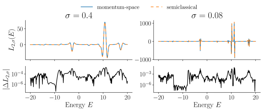
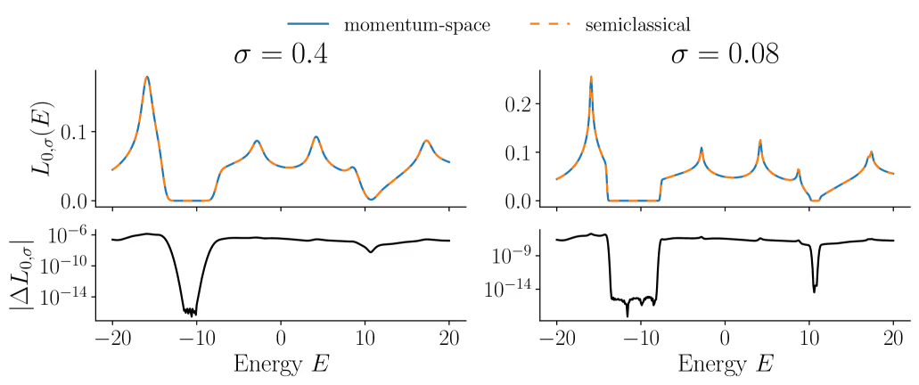
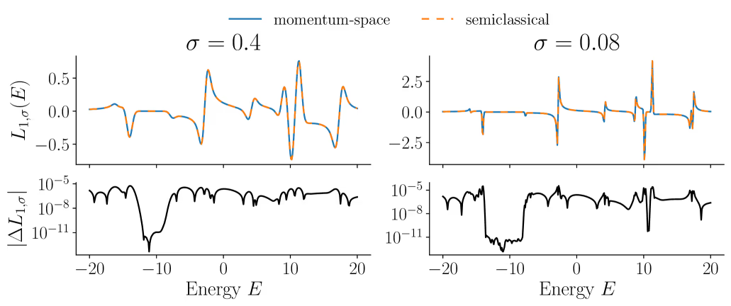
$\sigma=0.4$ and $\sigma=0.08$ , respectively, with momentum-space approximations of these functions obtained from a finite‐difference approximation in $\epsilon$ of the regularized DoS $\nu_{\epsilon,\sigma}$ computed from (2.10). As shown in Figures 1 to 3, the semiclassical and momentum-space approximations are in excellent agreement over the entire energy range.

Comparison of two numerical approximations of the function E↦L0,σ(E)E\mapsto L_{0,\sigma}(E) over the energy range −20 to 20-2020 for σ=0.4\sigma=0.4 (Left) and σ=0.08\sigma=0.08 (Right). The appr... — Figure 1: Comparison of two numerical approximations of the function $E\mapsto L_{0,\sigma}(E)$ over the energy range $-2020$ for $\sigma=0.4$ (Left) and $\sigma=0.08$ (Right). The approximations obtained by the momentum-space method are in solid blue, the ones obtained by discretization of the semiclassical formulae are in dashed orange, and the absolute errors between the two approximations are in black.

Comparison of two numerical approximations of the function E↦L1,σ(E)E\mapsto L_{1,\sigma}(E) over the energy range −20 to 20-2020 for σ=0.4\sigma=0.4 (Left) and σ=0.08\sigma=0.08 (Right). The appr... — Figure 2: Comparison of two numerical approximations of the function $E\mapsto L_{1,\sigma}(E)$ over the energy range $-2020$ for $\sigma=0.4$ (Left) and $\sigma=0.08$ (Right). The approximations obtained by the momentum-space method are in solid blue, the ones obtained by discretization of the semiclassical formulae are in dashed orange, and the absolute errors between the two approximations are in black.

Comparison of two numerical approximations of the function E↦L2,σ(E)E\mapsto L_{2,\sigma}(E) over the energy range −20 to 20-2020 for σ=0.4\sigma=0.4 (Left) and σ=0.08\sigma=0.08 (Right). The appr... — Figure 3: Comparison of two numerical approximations of the function $E\mapsto L_{2,\sigma}(E)$ over the energy range $-2020$ for $\sigma=0.4$ (Left) and $\sigma=0.08$ (Right). The approximations obtained by the momentum-space method are in solid blue, the ones obtained by discretization of the semiclassical formulae are in dashed orange, and the absolute errors between the two approximations are in black.

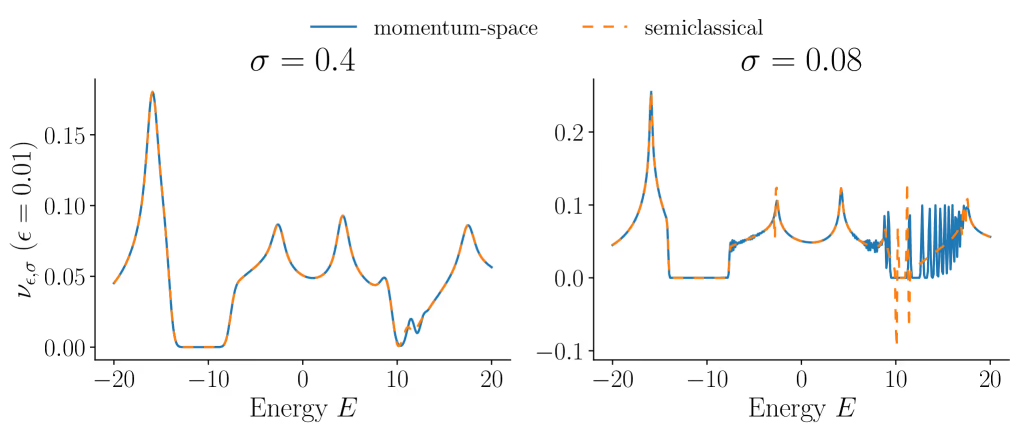
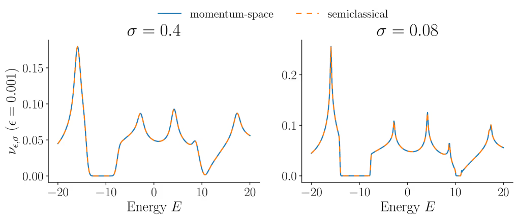
Next, we compare the approximations of the regularized density of states $\nu_{\epsilon,\sigma}$ obtained with (2.10) and (2.29) for two different values of $\epsilon$ ( $\epsilon=0.001$ and $\epsilon=0.01$ ) and two different values of $\sigma$ ( $\sigma=0.4$ and $\sigma=0.08$ ). In Figure 4, we observe that when $\epsilon$ is small enough (here $\epsilon=0.001$ ), there is strong agreement across the entire energy range. We further compare the momentum space/semiclassical approximations of $\nu_{\epsilon,\sigma}$ for a less small value of $\epsilon$ ( $\epsilon=0.01$ ) in Figure 5. We see that for $\sigma=0.4$ , slight differences appear around an energy value of 10; for $\sigma=0.08$ , significant differences occur in the range $[9,18]$ , along with minor differences in other energy ranges. In addition, we note that the approximations of $\nu_{\epsilon,\sigma}$ calculated using the momentum-space method exhibit pronounced oscillations in some energy ranges. The functions $L_{1,\sigma}$ and $L_{2,\sigma}$ displayed in Figures 2 and 3 also have dramatic changes in those energy ranges.

Comparison of the momentum space (solid blue) and second-order semiclassical (dashed orange) approximations of νϵ,σ\nu_{\epsilon,\sigma} of ϵ=0.001\epsilon=0.001 over the energy range −20 to 20-202... — Figure 4: Comparison of the momentum space (solid blue) and second-order semiclassical (dashed orange) approximations of $\nu_{\epsilon,\sigma}$ of $\epsilon=0.001$ over the energy range $-2020$ for $\sigma=0.4$ (Left) and ${\sigma=0.08}$ (Right).

Comparison of the momentum space (solid blue) and second-order semiclassical (dashed orange) approximations of νϵ,σ\nu_{\epsilon,\sigma} of ϵ=0.01\epsilon=0.01 over the energy range −20 to 20-2020 ... — Figure 5: Comparison of the momentum space (solid blue) and second-order semiclassical (dashed orange) approximations of $\nu_{\epsilon,\sigma}$ of $\epsilon=0.01$ over the energy range $-2020$ for $\sigma=0.4$ (Left) and ${\sigma=0.08}$ (Right).

3.3 Effective model for oscillations in DoS

Although the second-order semiclassical method fails to capture the fast oscillations of $\nu_{\epsilon,\sigma}$ , the semiclassical approach provides a qualitative, and even quantitative in the limit $|\epsilon|\ll 1$ , characterization of these oscillations.

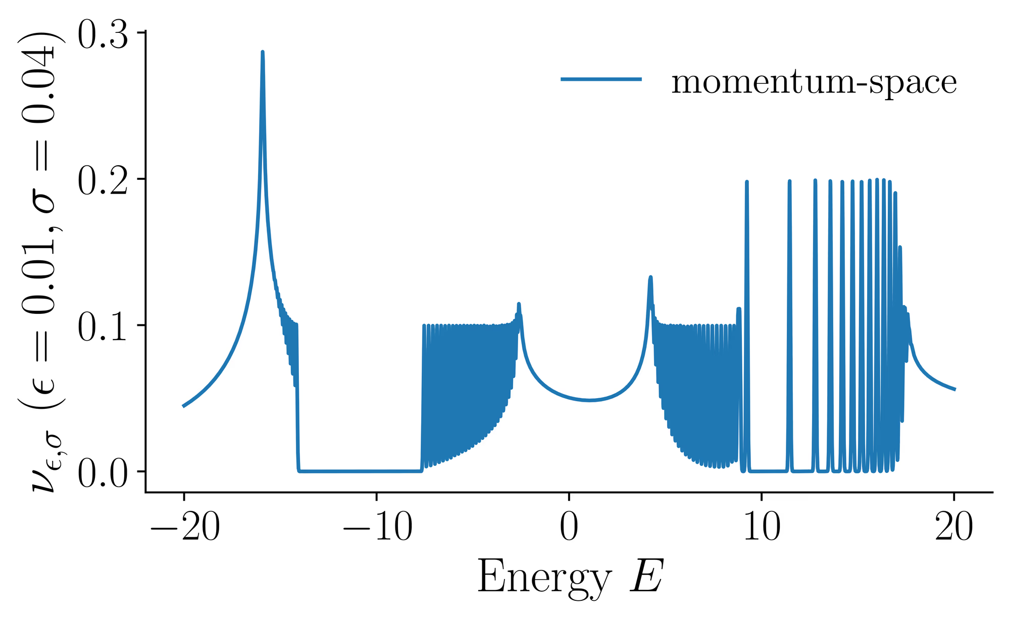
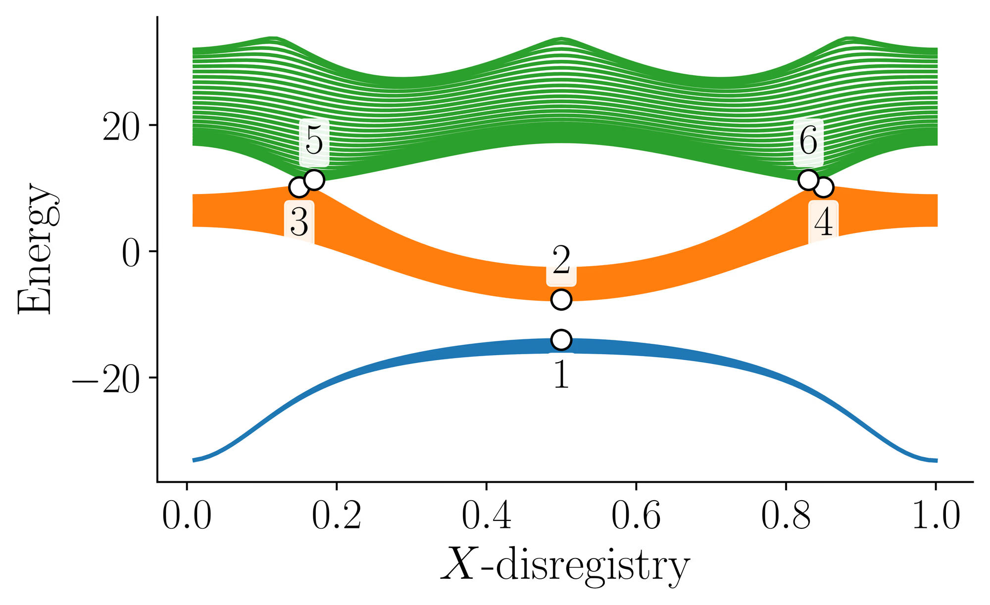
Let $E_{j}(k,X)$ be the $j$ -th eigenvalue of the operator $h(k,X)$ . As shown in Figure 6(a), the fast oscillations of $\nu_{\epsilon,\sigma}$ are localized in energy ranges close to critical values of the functions $E_{j}(k,X)$ , i.e., close to $E_{j}(k_{0},X_{0})$ where $(k_{0},X_{0})\in\Omega^{*}\times\Omega$ satisfies

\nabla_{k}E_{j}(k_{0},X_{0})=0\quad\mbox{and}\quad\nabla_{X}E_{j}(k_{0},X_{0})% =0\quad\mbox{for some }j.

These values are the analogue of Van Hove singularities in periodic systems [21].

For the sake of simplifying notation, we fix the band structure index $j$ and set $E(k,X)\coloneq E_{j}(k,X)$ in the following discussion. Let $P\subset\Omega^{*}\times\Omega$ be the set of the coordinates of the critical points of the band structures $(k,X)\mapsto E(k,X)$ . For each $p\coloneq(k_{0},X_{0})\in P$ , we have

E(k_{0}+\kappa,X_{0}+Y)\approx E(k_{0},X_{0})+\frac{1}{2}(A_{p}\kappa^{2}+2B_{% p}\kappa Y+C_{p}Y^{2}),

(3.4)

where

\displaystyle A_{p}\coloneq\frac{\partial^{2}E}{\partial k^{2}}(k_{0},X_{0}),% \quad B_{p}\coloneq\frac{\partial^{2}E}{\partial k\partial X}(k_{0},X_{0})% \quad\text{and}\quad C_{p}\coloneq\frac{\partial^{2}E}{\partial X^{2}}(k_{0},X% _{0}).

Table 1 lists the calculated parameters for the critical points $1$ to $6$ labeled in Figure 6(b), where $\omega_{p}$ is defined in (3.5) below. Note that $A_{p}C_{p}>0$ , so that these six critical points are either local minima or local maxima, and $B_{p}\approx 0$ for all these critical points. Assuming for simplicity that $B_{p}$ vanishes, the symbol in the RHS of (3.4) is a sum of a function of $\kappa$ and a function of $Y$ , so that its Weyl quantization $\left(\kappa\mapsto-i\frac{d}{dx},Y\mapsto\epsilon x\right)$ , is explicit, given by

\displaystyle H^{\rm eff}_{p}\coloneq{}

\displaystyle E(p)-\frac{1}{2}A_{p}\frac{d^{2}}{dx^{2}}+\frac{\epsilon^{2}}{2}% C_{p}x^{2}.

This is a quantum harmonic oscillator whose $n$ -th ( $n\in\mathbb{N}$ ) eigenvalue is

\displaystyle E_{p,n,\epsilon}\coloneq E(p)+\epsilon\,\omega_{p}\bigg(n+\frac{% 1}{2}\bigg)\quad\text{with}\quad\omega_{p}\coloneq\operatorname{sign}(A_{p})% \sqrt{A_{p}C_{p}}.

(3.5)

(a) Oscillations of νϵ,σ\nu_{\epsilon,\sigma} — (a) Oscillations of $\nu_{\epsilon,\sigma}$

(b) Band structures — (a) Oscillations of $\nu_{\epsilon,\sigma}$

Table 1: Energy, second-order derivatives, and oscillator angular frequency at critical points of the first three bands.

$p$	$E(p)$	$A_{p}$	$B_{p}$	$C_{p}$	$\omega_{p}$
1	$-14.046$	$-1.435$	$0.00$	$-132.008$	$-13.762$
2	$-7.662$	$2.618$	$0.00$	$210.261$	$23.461$
3 & 4	$10.133$	$-32.886$	$0.00$	$-1692.295$	$-235.907$
5 & 6	$11.287$	$36.267$	$0.00$	$1910.1673$	$263.204$

The harmonic approximation hence predicts a concentration of states at discrete energy levels at disregistries and momenta near the energies of the critical points $p$ . We note that such spectra are sometimes referred to as “flat bands” in the physics literature, despite not precisely corresponding to a constant energy band arising from Bloch theory. Similar situations can be seen, e.g., in the incommensurate double-walled carbon nanotube continuum model in [15] and the tight-binding model for TMDs in [6]. We note that the harmonic approximation predicts a collection of single flat bands, not the overlapping pair of flat bands seen in twisted bilayer graphene [3]. Then the approximation of the regularized DoS at the energy $E$ near the critical value $E(p)$ is calculated by

{\nu_{\epsilon,\sigma}(E)}\approx\frac{\epsilon}{|\Omega|}\sum_{\begin{% subarray}{c}p\in P\\ |E(p)-E|\ll 1\end{subarray}}\sum_{n\geq 0}\delta_{\sigma}\Bigg(E-E(p)-\omega_{% p}\epsilon\bigg(n+\frac{1}{2}\bigg)\Bigg).

(3.6)

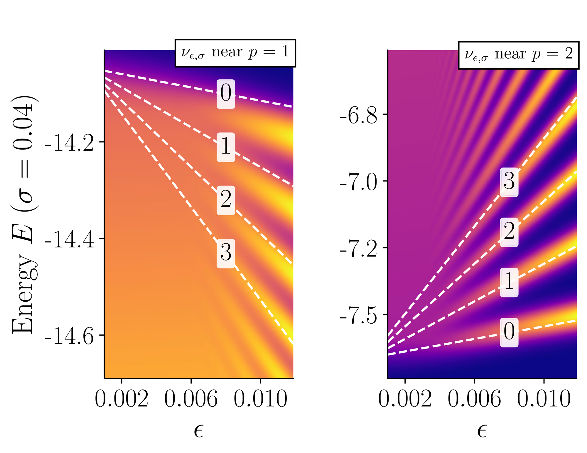
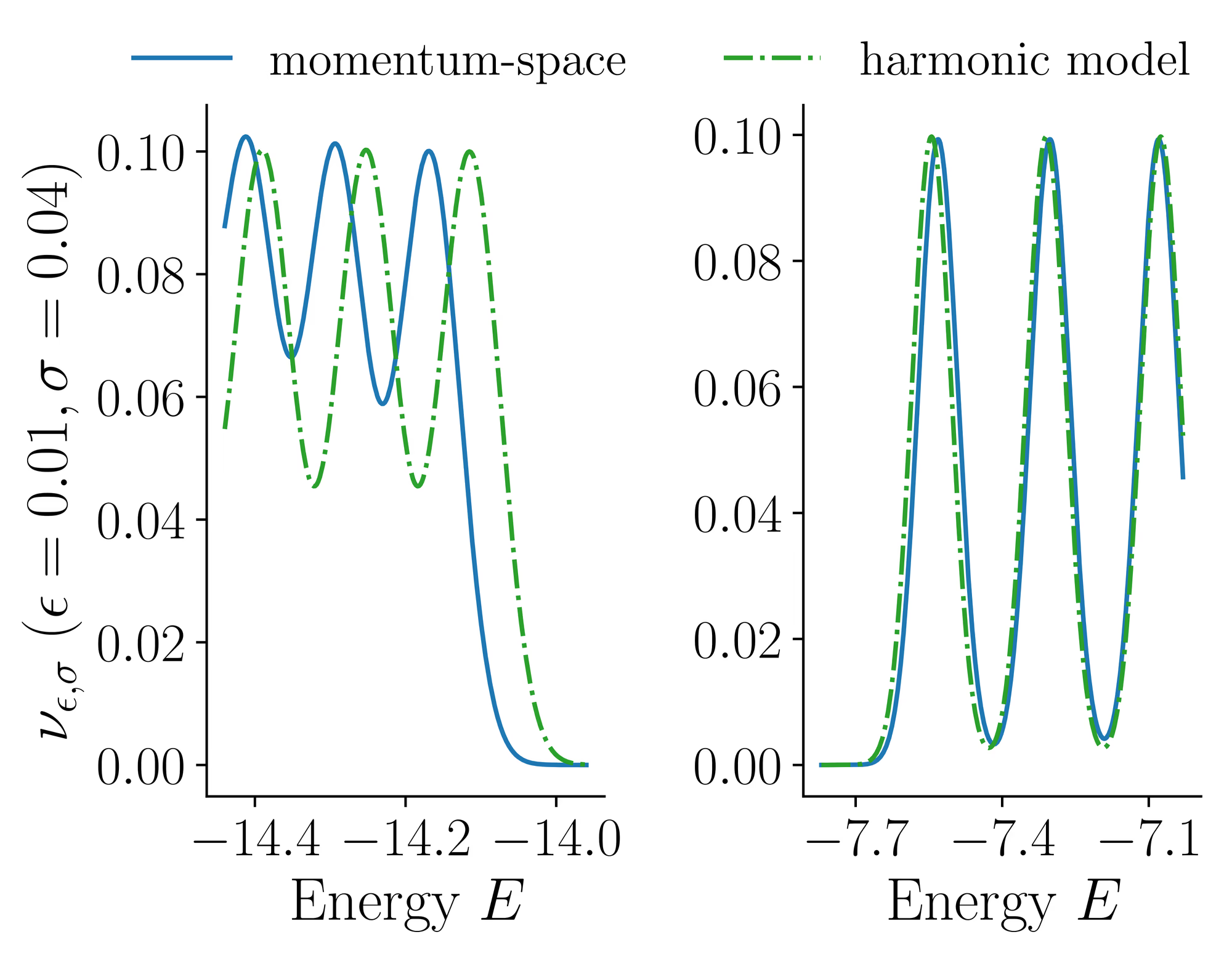
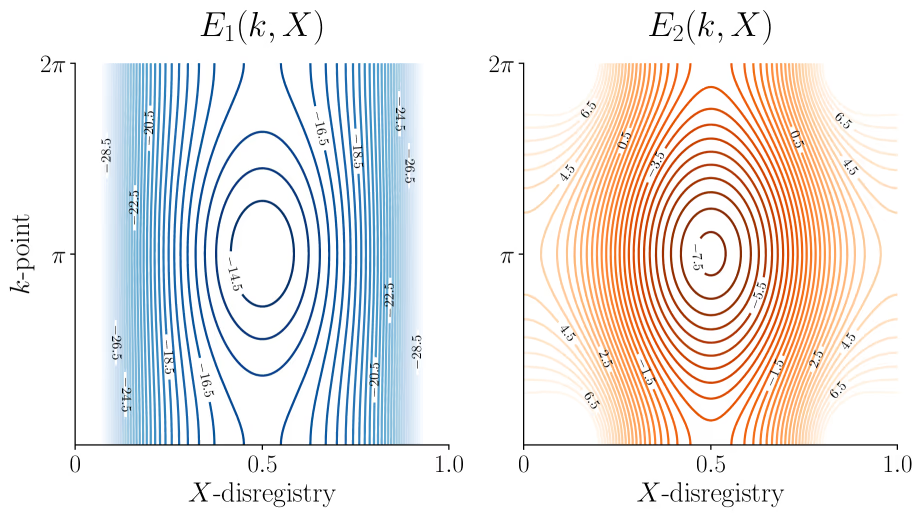
We first verify the applicability of the harmonic approximation for critical points 1 and 2, both of which are located in relatively flat regions of the band structures. In Figure 7, we compare the approximation of the regularized DoS calculated by the momentum-space method (2.10) for $\sigma=0.04$ with two predictions of the harmonic approximation: (a) the expected energy levels from (3.5) for $\epsilon$ in $[0.001,0.011]$ , and (b) the approximation of the regularized DoS given by (3.6) for $\epsilon=0.01$ . We observe excellent agreement between the momentum-space calculation and the harmonic approximation for $p=2$ , while the agreement is not as good for $p=1$ . This difference can be explained by analyzing the level sets of the functions $(k,X)\mapsto E_{j}(k,X)$ , $j=1,2$ , which are plotted in Figure 8. The idea is that if the normalized eigenstates $u_{\epsilon,n}\in L^{2}(\mathbb{R})$ , $n=0,1,2,\cdots,n_{0}-1$ of the effective harmonic Hamiltonian around $E(p)$ are localized in the region where the harmonic approximation is valid, the first $n_{0}$ oscillations should be well-described by $H^{\rm eff}_{p}$ . To quantify this criterion, it is convenient to introduce the Wigner transform of the (shifted and rescaled) eigenstates $u_{\epsilon,n}$ , given by

\displaystyle\mathcal{W}(u_{n,\epsilon})(k,X)\coloneq\frac{1}{\pi\hbar}\int_{% \mathbb{R}}u_{\epsilon,n}^{*}\bigg(\frac{X-X_{0}}{\epsilon}+y\bigg)u_{\epsilon% ,n}\bigg(\frac{X-X_{0}}{\epsilon}-y\bigg)e^{2i\hbar^{-1}(k-k_{0})y}\,dy,\qquad% \hbar=1.

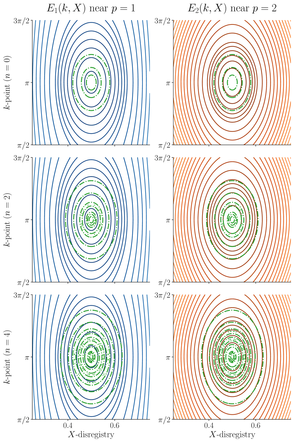
Remarkably, the Wigner transform of an eigenfunction of a 1D quantum harmonic oscillator is constant over the level sets of the corresponding classical Hamiltonian (see e.g., [19, 24]). Plotting the level sets of $|\mathcal{W}(u_{n,\epsilon})(k,X)|$ associated with non-negligible values on top of the level sets of $E(k,X)$ , we can expect the harmonic approximation will give satisfactory results if, in the regions of the phase space where $|\mathcal{W}(u_{n,\epsilon})(k,X)|$ is not small, this function takes almost constant values on the level sets of $E(k,X)$ . A careful examination of the plots in Figure 9 shows that this is the case for the eigenstates $n=0,2,4$ of $H^{\rm eff}_{p=2}$ , but not really for the eigenstates $n=0,2,4$ of $H^{\rm eff}_{p=1}$ . These observations further explain why, for $\epsilon=0.01$ , the harmonic approximation is less accurate for $p=1$ than for $p=2$ .

Level sets of (k,X)↦Ej(k,X)(k,X)\mapsto E_{j}(k,X) for j=1j=1 (Left) and j=2j=2 (Right). — Figure 8: Level sets of $(k,X)\mapsto E_{j}(k,X)$ for $j=1$ (Left) and $j=2$ (Right).

Comparison of the level sets of E(k,X)E(k,X) with the level sets of |𝒲(un,ϵ)(X,k)||\mathcal{W}(u_{n,\epsilon})(X,k)| (dashed green contours) for ϵ=0.01\epsilon=0.01 and n=0,2,4n=0,2,4, showing t... — Figure 9: Comparison of the level sets of $E(k,X)$ with the level sets of $|\mathcal{W}(u_{n,\epsilon})(X,k)|$ (dashed green contours) for $\epsilon=0.01$ and $n=0,2,4$ , showing the regions surrounding $p=1$ (Left) and $p=2$ (Right). The parameters of the eigenstates are listed in Table 1.

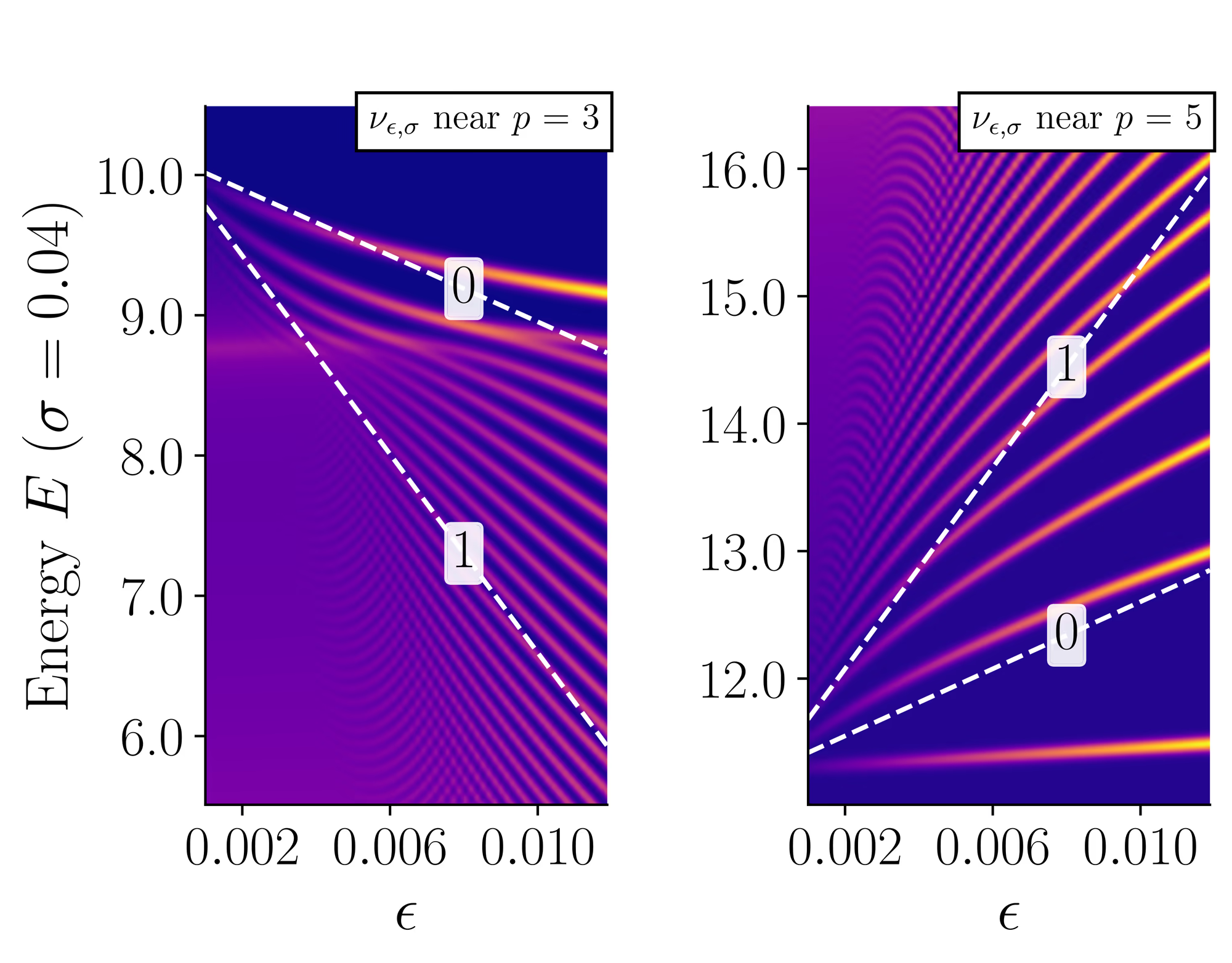
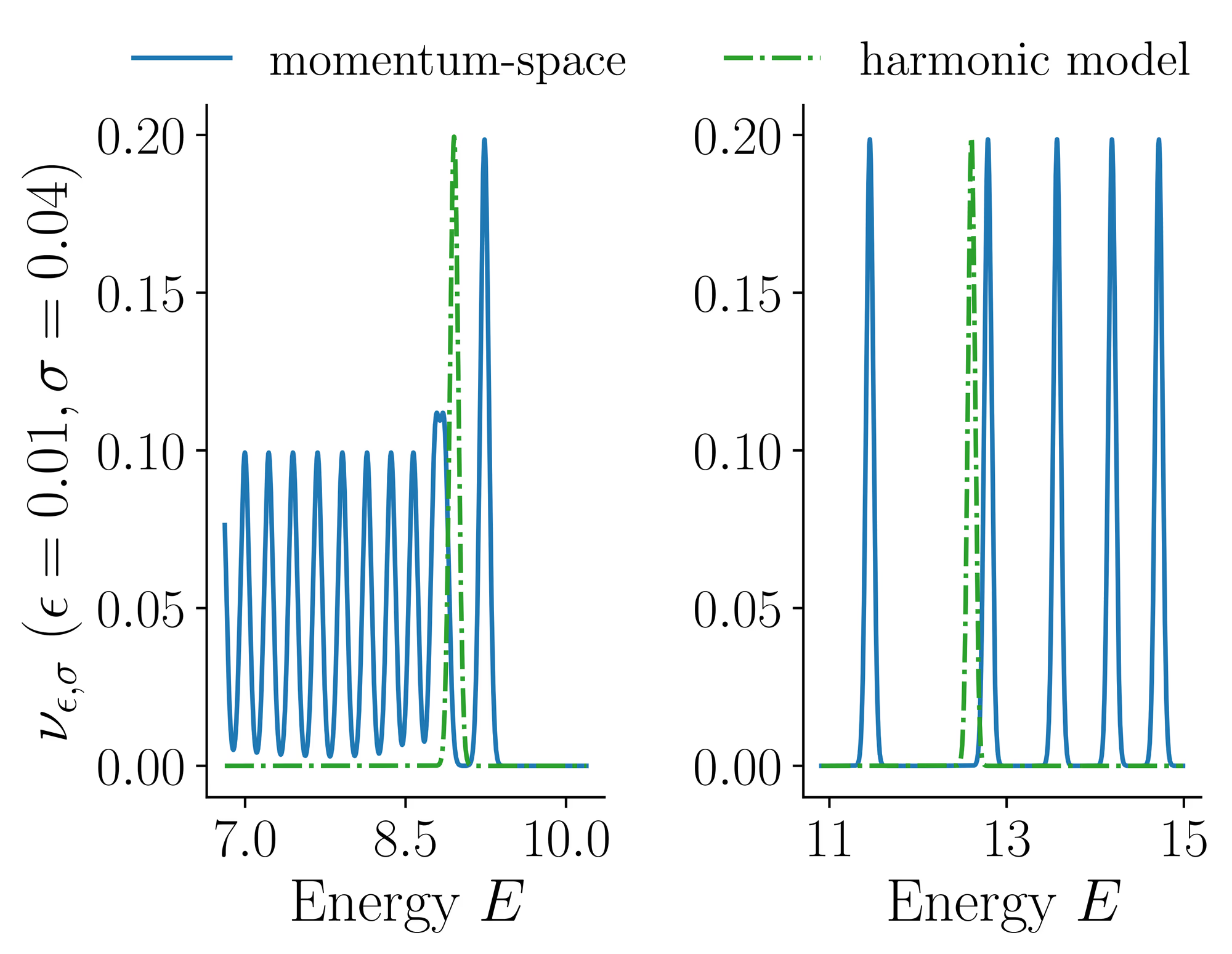
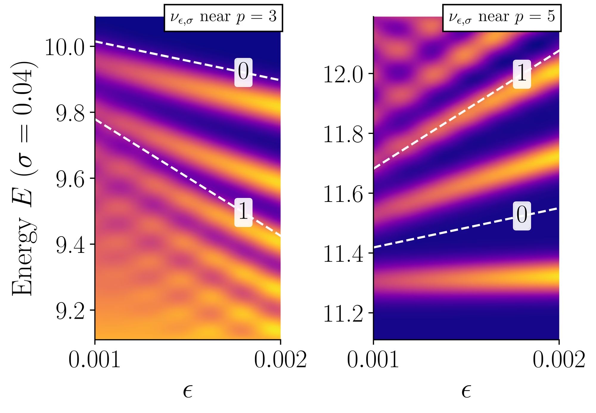
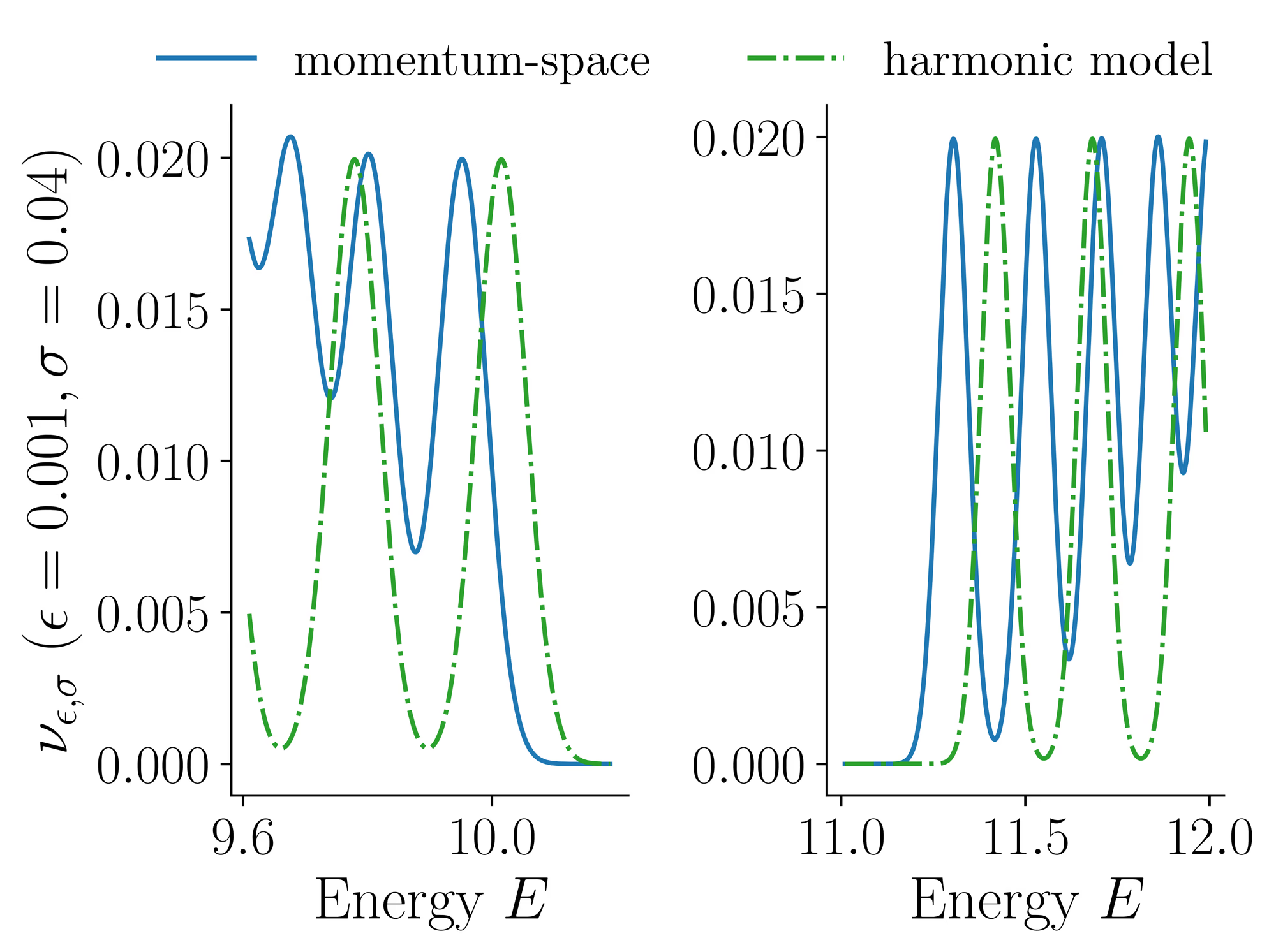
We next present results for $p=3$ to $6$ in the same $\epsilon$ regimes. Here, we focus on $p=3$ and $p=5$ , as the results for $p=4$ and $p=6$ are identical due to the symmetry of the band structures. As shown in Figure 10, the harmonic approximation exhibits significant deviations from the momentum-space calculation. Figure 6(b) shows that the band structures near $p=3$ and $p=5$ are much steeper than those near $p=1$ and $p=2$ . In addition, the local gaps between the second and third bands around $p=3$ and $p=5$ are much smaller than the local gaps between the first and second bands around $p=1$ and $p=2$ , leading to non-negligible coupling between bands $2$ and $3$ at the moiré scale at energy around $10$ . While a single band harmonic approximation around $p=1$ and $p=2$ suffices to capture the main features of the DoS in the corresponding energy ranges for the considered values of $\epsilon$ , this is not the case for $p=3$ and $p=5$ .

Although the harmonic approximations around $p=3$ to $6$ rapidly deviate from the momentum-space approximation of the regularized DoS as $\epsilon$ increases across the range $[0.001,0.011]$ , we see in Figure 11 that the two methods still exhibit good agreement for sufficiently small values of $\epsilon$ within this range. From Table 1, we note that the oscillator angular frequency $\omega_{p}$ is small for $p=1,2$ and large for $p=3$ to $6$ . According to the eigenvalue approximation (3.5), a large $\omega_{p}$ causes the eigenvalues $E_{p,n,\epsilon}$ to grow rapidly with $\epsilon$ . In addition, note that the effective supports of the Wigner transforms of $u_{n,\epsilon}$ depends on $\epsilon\frac{\omega_{p}}{A_{p}}$ , although the values of $\frac{\omega_{p}}{A_{p}}$ differ only slightly for $p=1$ to 6, a pronounced steepness is observed in the band structures near $p=3$ and $5$ . Therefore, the harmonic oscillator model remains valid only for very small values of $\epsilon$ around critical points $p=3,5$ .

4 Conclusion

In this paper, we have investigated two different methods for approximating the density of states of incommensurate Hamiltonians: a momentum-space method (Section 2.1) and a semiclassical expansion method (Section 2.2). Using a simple 1D toy model and Gaussian smearing, we compared the approximations of the regularized DoS $\nu_{\epsilon,\sigma}$ computed by these two methods. We first check the consistency of these two methods by comparing the first three terms of the asymptotic expansion in $|\epsilon|\ll 1$ of $\nu_{\epsilon,\sigma}$ . Then, we compare the approximations of $\nu_{\epsilon,\sigma}$ for different values of $\epsilon$ and $\sigma$ . We observe that, when truncated the semiclassical expansion after second-order, the methods exhibit excellent agreement in the small $\epsilon$ regime, while discrepancies arise for less small $\epsilon$ . This indicates the importance of higher-order corrections in the semiclassical method for such regimes. These discrepancies are mainly caused by oscillations in the DoS, which can be analyzed using semiclassical techniques.

Acknowledgments

This project has received funding from the Simons Targeted Grant Award No. 896630 and from the European Research Council (ERC) under the European Union’s Horizon 2020 research and innovation programme (grant agreement EMC2 No 810367). DM’s research was supported by AFRL grant FA9550-24-1-0177.

Appendix A Derivation of formulae (2.26) and (2.27)

In this section, we prove Theorem 2.5 from the semiclassical formulae (2.21)-(2.23) (derived as in [4]) and the spectral decomposition (2.24). It is easy to see that Eq. (2.25) follows immediately from (2.21). Thus we only focus on the derivation of (2.26) and (2.27) from (2.22) and (2.23) respectively.

A.1 Proof of (2.26)

We first decompose $(z-h)^{-1}\{(z-h),(z-h)^{-1}\}$ by using (2.24). From

\displaystyle\{(z-h),(z-h)^{-1}\}=\nabla_{k}h\cdot(z-h)^{-1}\nabla_{X}h(z-h)^{% -1}-\nabla_{X}h\cdot(z-h)^{-1}\nabla_{k}h(z-h)^{-1},

we get

	$\displaystyle(z-h)^{-1}\{(z-h),(z-h)^{-1}\}$
	$\displaystyle=(z-h)^{-1}\nabla_{k}h\cdot(z-h)^{-1}\nabla_{X}h(z-h)^{-1}-(z-h)^% {-1}\cdot\nabla_{X}h(z-h)^{-1}\nabla_{k}h(z-h)^{-1}.$

Using the fact that $\mathcal{K}_{mn}=\overline{\mathcal{K}}_{nm}$ and $\mathcal{X}_{mn}=\overline{\mathcal{X}}_{nm}$ , we get

\displaystyle\operatorname{Tr}_{L^{2}_{\rm per}}[\{(z-h)^{-1},(z-h)\}(z-h)^{-1% }]=2i\sum_{m,n}(\zeta-\lambda_{m})^{-2}(\zeta-\lambda_{n})^{-1}\operatorname{% Im}(\mathcal{K}_{mn}\cdot\mathcal{X}_{nm}),

from which we get

\displaystyle\operatorname{Tr}_{L^{2}_{\rm per}}[f_{1}]

\displaystyle=-\frac{1}{2}\sum_{m,n}f_{2}^{(2)}(\lambda_{m};\lambda_{n})% \operatorname{Im}(\mathcal{K}_{mn}\cdot\mathcal{X}_{nm}).

This gives

\displaystyle L_{1}(f)=-\frac{1}{2(2\pi)^{d}}\sum_{m,n}\fint_{\Omega}\int_{% \Omega^{*}}f_{2}^{(2)}(\lambda_{m}(k,X);\lambda_{n}(k,X))\operatorname{Im}(% \mathcal{K}_{mn}(k,X)\cdot\mathcal{X}_{nm}(k,X))\,dk\,dX.

A.2 Proof of (2.27)

First, we observe that

	$\displaystyle(z-h)^{-1}\{(z-h),(z-h)^{-1}\{(z-h),(z-h)^{-1}\}\}$
	$\displaystyle=(z-h)^{-1}\{(z-h),(z-h)^{-1}\}\{(z-h),(z-h)^{-1}\}$
	$\displaystyle+(z-h)^{-1}\nabla_{X}(z-h)(z-h)^{-1}\cdot\nabla_{k}\{(z-h),(z-h)^% {-1}\}$
	$\displaystyle-(z-h)^{-1}\nabla_{k}(z-h)(z-h)^{-1}\cdot\nabla_{X}\{(z-h),(z-h)^% {-1}\}$
	$\displaystyle=(z-h)^{-1}\{(z-h),(z-h)^{-1}\}^{2}-\{(z-h)^{-1},\{(z-h),(z-h)^{-% 1}\}\}.$

Thus,

\displaystyle\operatorname{Tr}_{L^{2}_{\rm per}}[f_{2}](k,X)=I(k,X)+II(k,X)+% III(k,X),

with

	$\displaystyle I$	$\displaystyle\coloneq-\frac{1}{\pi}\int_{\mathbb{C}}\overline{\partial}% \widetilde{f}(z)\Big[-\frac{1}{4}\operatorname{Tr}_{L^{2}_{\rm per}}[(z-h)^{-1% }\{(z-h),(z-h)^{-1}\}^{2}]\Big]\,dL(z)$
	$\displaystyle II$	$\displaystyle\coloneq-\frac{1}{\pi}\int_{\mathbb{C}}\overline{\partial}% \widetilde{f}(z)\Big[\frac{1}{4}\operatorname{Tr}_{L^{2}_{\rm per}}[\{(z-h)^{-% 1},\{(z-h),(z-h)^{-1}\}\}]\Big]\,dL(z)$
	$\displaystyle III$	$\displaystyle\coloneq-\frac{1}{\pi}\int_{\mathbb{C}}\overline{\partial}% \widetilde{f}(z)\Big[\frac{1}{8}\operatorname{Tr}_{L^{2}_{\rm per}}[(z-h)^{-1}% \{(z-h),(z-h)^{-1}\}_{2}]\Big]\,dL(z).$

A.2.1 Reformulation of $I$

As

\displaystyle\{(z-h),(z-h)^{-1}\}=\nabla_{k}h\cdot(z-h)^{-1}\nabla_{X}h(z-h)^{% -1}-\nabla_{X}h\cdot(z-h)^{-1}\nabla_{k}h(z-h)^{-1},

we have

	$\displaystyle(z-h)^{-1}\{(z-h),(z-h)^{-1}\}^{2}$
	$\displaystyle=(z-h)^{-1}\Big(\nabla_{k}h\cdot(z-h)^{-1}\nabla_{X}h\Big)(z-h)^{% -1}\Big(\nabla_{k}h\cdot(z-h)^{-1}\nabla_{X}h\Big)(z-h)^{-1}$
	$\displaystyle\quad+(z-h)^{-1}\Big(\nabla_{X}h\cdot(z-h)^{-1}\nabla_{k}h\Big)(z% -h)^{-1}\Big(\nabla_{X}h\cdot(z-h)^{-1}\nabla_{k}h\Big)(z-h)^{-1}$
	$\displaystyle\quad-(z-h)^{-1}\Big(\nabla_{k}h\cdot(z-h)^{-1}\nabla_{X}h\Big)(z% -h)^{-1}\Big(\nabla_{X}h\cdot(z-h)^{-1}\nabla_{k}h\Big)(z-h)^{-1}$
	$\displaystyle\quad-(z-h)^{-1}\Big(\nabla_{X}h\cdot(z-h)^{-1}\nabla_{k}h\Big)(z% -h)^{-1}\Big(\nabla_{k}h\cdot(z-h)^{-1}\nabla_{X}h\Big)(z-h)^{-1}$
	$\displaystyle\eqcolon I_{1}(z)+I_{2}(z)+I_{3}(z)+I_{4}(z).$

Using the spectral decomposition (2.24), we obtain

	$\displaystyle-\frac{1}{\pi}\int_{\mathbb{C}}\overline{\partial}\widetilde{f}(% \zeta)\operatorname{Tr}_{L^{2}_{\rm per}}[I_{1}(z)]\,dL(\zeta)$	$\displaystyle=\frac{1}{4!}\sum_{m,n,p,q}f_{4}^{(4)}(\lambda_{m};\lambda_{n},% \lambda_{p},\lambda_{q})(\mathcal{K}_{mn}\cdot\mathcal{X}_{np})(\mathcal{K}_{% pq}\cdot\mathcal{X}_{qm}),$
	$\displaystyle-\frac{1}{\pi}\int_{\mathbb{C}}\overline{\partial}\widetilde{f}(% \zeta)\operatorname{Tr}_{L^{2}_{\rm per}}[I_{2}(z)]\,dL(\zeta)$	$\displaystyle=\frac{1}{4!}\sum_{m,n,p,q}f_{4}^{(4)}(\lambda_{m};\lambda_{n},% \lambda_{p},\lambda_{q})(\mathcal{X}_{mn}\cdot\mathcal{K}_{np})(\mathcal{X}_{% pq}\cdot\mathcal{K}_{qm}),$
	$\displaystyle-\frac{1}{\pi}\int_{\mathbb{C}}\overline{\partial}\widetilde{f}(% \zeta)\operatorname{Tr}_{L^{2}_{\rm per}}[I_{3}(z)]\,dL(\zeta)$	$\displaystyle=-\frac{1}{4!}\sum_{m,n,p,q}f_{4}^{(4)}(\lambda_{m};\lambda_{n},% \lambda_{p},\lambda_{q})(\mathcal{K}_{mn}\cdot\mathcal{X}_{np})(\mathcal{X}_{% pq}\cdot\mathcal{K}_{qm}),$
	$\displaystyle-\frac{1}{\pi}\int_{\mathbb{C}}\overline{\partial}\widetilde{f}(% \zeta)\operatorname{Tr}_{L^{2}_{\rm per}}[I_{4}(z)]\,dL(\zeta)$	$\displaystyle=-\frac{1}{4!}\sum_{m,n,p,q}f_{4}^{(4)}(\lambda_{m};\lambda_{n},% \lambda_{p},\lambda_{q})(\mathcal{X}_{mn}\cdot\mathcal{K}_{np})(\mathcal{K}_{% pq}\cdot\mathcal{X}_{qm}).$

By symmetry, we get

		$\displaystyle I=\frac{1}{96}\sum_{m,n,p,q}f_{4}^{(4)}(\lambda_{m};\lambda_{n},% \lambda_{p},\lambda_{q})\Big[-2\operatorname{Re}\Big((\mathcal{K}_{mn}\cdot% \mathcal{X}_{np})(\mathcal{K}_{pq}\cdot\mathcal{X}_{qm})\Big)$
		$\displaystyle\hskip 113.81102pt+(\mathcal{K}_{mn}\cdot\mathcal{X}_{np})(% \mathcal{X}_{pq}\cdot\mathcal{K}_{qm})+(\mathcal{X}_{mn}\cdot\mathcal{K}_{np})% (\mathcal{K}_{pq}\cdot\mathcal{X}_{qm})\Big].$		(A.1)

A.2.2 Reformulation of $II$

We have for $l=1,\dots,d$ ,

	$\displaystyle\partial_{k_{l}}\{(z-h),(z-h)^{-1}\}$
	$\displaystyle=\partial_{k_{l}}\sum_{j}\left(\partial_{k_{j}}h\partial_{X_{j}}(% z-h)^{-1}-\partial_{X_{j}}h\partial_{k_{j}}(z-h)^{-1}\right)$
	$\displaystyle=(z-h)^{-1}\partial_{X_{l}}h(z-h)^{-1}-\partial_{X_{l}}h(z-h)^{-2}$
	$\displaystyle\quad+\sum_{j}\partial_{k_{j}}h(z-h)^{-1}\partial_{k_{l}}h(z-h)^{% -1}\partial_{X_{j}}h(z-h)^{-1}$
	$\displaystyle\quad+\sum_{j}\partial_{k_{j}}h(z-h)^{-1}\partial_{X_{j}}h(z-h)^{% -1}\partial_{k_{l}}h(z-h)^{-1}$
	$\displaystyle\quad-\sum_{j}\partial_{X_{j}}h(z-h)^{-1}\partial_{k_{j}}h(z-h)^{% -1}\partial_{k_{l}}h(z-h)^{-1}$
	$\displaystyle\quad-\sum_{j}\partial_{X_{j}}h(z-h)^{-1}\partial_{k_{l}}h(z-h)^{% -1}\partial_{k_{j}}h(z-h)^{-1},$

and

	$\displaystyle\partial_{X_{l}}\{(z-h),(z-h)^{-1}\}$
	$\displaystyle=\partial_{X_{l}}\sum_{j}\left(\partial_{k_{j}}h\partial_{X_{j}}(% z-h)^{-1}-\partial_{X_{j}}h\partial_{k_{j}}(z-h)^{-1}\right)$
	$\displaystyle=\sum_{j}\partial_{k_{j}}h(z-h)^{-1}\partial_{X_{j}}h(z-h)^{-1}% \partial_{X_{l}}h(z-h)^{-1}$
	$\displaystyle\quad+\sum_{j}\partial_{k_{j}}h(z-h)^{-1}\partial_{X_{l}}h(z-h)^{% -1}\partial_{X_{j}}h(z-h)^{-1}$
	$\displaystyle\quad+\sum_{j}\partial_{k_{j}}h(z-h)^{-1}\partial_{X_{j}}\partial% _{X_{l}}h(z-h)^{-1}$
	$\displaystyle\quad-\sum_{j}\partial_{X_{j}}\partial_{X_{l}}h(z-h)^{-1}\partial% _{k_{j}}h(z-h)^{-1}$
	$\displaystyle\quad-\sum_{j}\partial_{X_{j}}h(z-h)^{-1}\partial_{X_{l}}h(z-h)^{% -1}\partial_{k_{j}}h(z-h)^{-1}$
	$\displaystyle\quad-\sum_{j}\partial_{X_{j}}h(z-h)^{-1}\partial_{k_{j}}h(z-h)^{% -1}\partial_{X_{l}}h(z-h)^{-1}.$

As a result, we have

	$\displaystyle\nabla_{X}(z-h)^{-1}\cdot\nabla_{k}\{(z-h),(z-h)^{-1}\}$
	$\displaystyle=\sum_{l}(z-h)^{-1}\partial_{X_{l}}h(z-h)^{-2}\partial_{X_{l}}h(z% -h)^{-1}$
	$\displaystyle\quad-\sum_{l}(z-h)^{-1}\partial_{X_{l}}h(z-h)^{-1}\partial_{X_{l% }}h(z-h)^{-2}$
	$\displaystyle\quad+\sum_{j,l}(z-h)^{-1}\partial_{X_{l}}h(z-h)^{-1}\partial_{k_% {j}}h(z-h)^{-1}\partial_{k_{l}}h(z-h)^{-1}\partial_{X_{j}}h(z-h)^{-1}$
	$\displaystyle\quad+\sum_{j,l}(z-h)^{-1}\partial_{X_{l}}h(z-h)^{-1}\partial_{k_% {j}}h(z-h)^{-1}\partial_{X_{j}}h(z-h)^{-1}\partial_{k_{l}}h(z-h)^{-1}$
	$\displaystyle\quad-\sum_{j,l}(z-h)^{-1}\partial_{X_{l}}h(z-h)^{-1}\partial_{X_% {j}}h(z-h)^{-1}\partial_{k_{j}}h(z-h)^{-1}\partial_{k_{l}}h(z-h)^{-1}$
	$\displaystyle\quad-\sum_{j,l}(z-h)^{-1}\partial_{X_{l}}h(z-h)^{-1}\partial_{X_% {j}}h(z-h)^{-1}\partial_{k_{l}}h(z-h)^{-1}\partial_{k_{j}}h(z-h)^{-1}$
	$\displaystyle\eqcolon II_{1}(z)+II_{2}(z)+II_{3}(z)+II_{4}(z)+II_{5}(z)+II_{6}% (z),$

and

	$\displaystyle-\nabla_{k}(z-h)^{-1}\cdot\nabla_{X}\{(z-h),(z-h)^{-1}\}$
	$\displaystyle=-\sum_{j,l}(z-h)^{-1}\partial_{k_{l}}h(z-h)^{-1}\partial_{k_{j}}% h(z-h)^{-1}\partial_{X_{j}}h(z-h)^{-1}\partial_{X_{l}}h(z-h)^{-1}$
	$\displaystyle\quad-\sum_{j,l}(z-h)^{-1}\partial_{k_{l}}h(z-h)^{-1}\partial_{k_% {j}}h(z-h)^{-1}\partial_{X_{l}}h(z-h)^{-1}\partial_{X_{j}}h(z-h)^{-1}$
	$\displaystyle\quad-\sum_{j,l}(z-h)^{-1}\partial_{k_{l}}h(z-h)^{-1}\partial_{k_% {j}}h(z-h)^{-1}\partial_{X_{j}}\partial_{X_{l}}h(z-h)^{-1}$
	$\displaystyle\quad+\sum_{j,l}(z-h)^{-1}\partial_{k_{l}}h(z-h)^{-1}\partial_{X_% {j}}\partial_{X_{l}}h(z-h)^{-1}\partial_{k_{j}}h(z-h)^{-1}$
	$\displaystyle\quad+\sum_{j,l}(z-h)^{-1}\partial_{k_{l}}h(z-h)^{-1}\partial_{X_% {j}}h(z-h)^{-1}\partial_{X_{l}}h(z-h)^{-1}\partial_{k_{j}}h(z-h)^{-1}$
	$\displaystyle\quad+\sum_{j,l}(z-h)^{-1}\partial_{k_{l}}h(z-h)^{-1}\partial_{X_% {j}}h(z-h)^{-1}\partial_{k_{j}}h(z-h)^{-1}\partial_{X_{l}}h(z-h)^{-1}$
	$\displaystyle\eqcolon II_{7}(z)+II_{8}(z)+II_{9}(z)+II_{10}(z)+II_{11}(z)+II_{% 12}(z).$

Using again (2.24), we obtain

	$\displaystyle-\frac{1}{\pi}\int_{\mathbb{C}}\overline{\partial}\widetilde{f}(% \zeta)\operatorname{Tr}_{L^{2}_{\rm per}}[II_{1}(z)]\,dL(\zeta)$	$\displaystyle=\frac{1}{3!}\sum_{m,n}f^{(3)}_{3}(\lambda_{m};\lambda_{n},% \lambda_{n})\|\mathcal{X}_{mn}\|^{2}$
	$\displaystyle-\frac{1}{\pi}\int_{\mathbb{C}}\overline{\partial}\widetilde{f}(% \zeta)\operatorname{Tr}_{L^{2}_{\rm per}}[II_{2}(z)]\,dL(\zeta)$	$\displaystyle=-\frac{1}{3!}\sum_{m,n}f_{3}^{(3)}(\lambda_{m};\lambda_{m},% \lambda_{n})\|\mathcal{X}_{mn}\|^{2}$
	$\displaystyle-\frac{1}{\pi}\int_{\mathbb{C}}\overline{\partial}\widetilde{f}(% \zeta)\operatorname{Tr}_{L^{2}_{\rm per}}[II_{3}(z)]\,dL(\zeta)$	$\displaystyle=\frac{1}{4!}\sum_{m,n,p,q}f^{(4)}_{4}(\lambda_{m};\lambda_{n},% \lambda_{p},\lambda_{q})(\mathcal{X}_{mn}\cdot\mathcal{K}_{pq})(\mathcal{K}_{% np}\cdot\mathcal{X}_{qm})$
	$\displaystyle-\frac{1}{\pi}\int_{\mathbb{C}}\overline{\partial}\widetilde{f}(% \zeta)\operatorname{Tr}_{L^{2}_{\rm per}}[II_{4}(z)]\,dL(\zeta)$	$\displaystyle=\frac{1}{4!}\sum_{m,n,p,q}f^{(4)}_{4}(\lambda_{m};\lambda_{n},% \lambda_{p},\lambda_{q})(\mathcal{X}_{mn}\cdot\mathcal{K}_{qm})(\mathcal{K}_{% np}\cdot\mathcal{X}_{pq})$
	$\displaystyle-\frac{1}{\pi}\int_{\mathbb{C}}\overline{\partial}\widetilde{f}(% \zeta)\operatorname{Tr}_{L^{2}_{\rm per}}[II_{5}(z)]\,dL(\zeta)$	$\displaystyle=-\frac{1}{4!}\sum_{m,n,p,q}f^{(4)}_{4}(\lambda_{m};\lambda_{n},% \lambda_{p},\lambda_{q})(\mathcal{X}_{mn}\cdot\mathcal{K}_{qm})(\mathcal{X}_{% np}\cdot\mathcal{K}_{pq})$
	$\displaystyle-\frac{1}{\pi}\int_{\mathbb{C}}\overline{\partial}\widetilde{f}(% \zeta)\operatorname{Tr}_{L^{2}_{\rm per}}[II_{6}(z)]\,dL(\zeta)$	$\displaystyle=-\frac{1}{4!}\sum_{m,n,p,q}f^{(4)}_{4}(\lambda_{m};\lambda_{n},% \lambda_{p},\lambda_{q})(\mathcal{X}_{mn}\cdot\mathcal{K}_{pq})(\mathcal{X}_{% np}\cdot\mathcal{K}_{qm})$
	$\displaystyle-\frac{1}{\pi}\int_{\mathbb{C}}\overline{\partial}\widetilde{f}(% \zeta)\operatorname{Tr}_{L^{2}_{\rm per}}[II_{7}(z)]\,dL(\zeta)$	$\displaystyle=-\frac{1}{4!}\sum_{m,n,p,q}f^{(4)}_{4}(\lambda_{m};\lambda_{n},% \lambda_{p},\lambda_{q})(\mathcal{K}_{mn}\cdot\mathcal{X}_{qm})(\mathcal{K}_{% np}\cdot\mathcal{X}_{pq})$
	$\displaystyle-\frac{1}{\pi}\int_{\mathbb{C}}\overline{\partial}\widetilde{f}(% \zeta)\operatorname{Tr}_{L^{2}_{\rm per}}[II_{8}(z)]\,dL(\zeta)$	$\displaystyle=-\frac{1}{4!}\sum_{m,n,p,q}f^{(4)}_{4}(\lambda_{m};\lambda_{n},% \lambda_{p},\lambda_{q})(\mathcal{K}_{mn}\cdot\mathcal{X}_{pq})(\mathcal{K}_{% np}\cdot\mathcal{X}_{qm})$
	$\displaystyle-\frac{1}{\pi}\int_{\mathbb{C}}\overline{\partial}\widetilde{f}(% \zeta)\operatorname{Tr}_{L^{2}_{\rm per}}[II_{9}(z)]\,dL(\zeta)$	$\displaystyle=-\frac{1}{3!}\sum_{m,n,p}f^{(3)}_{3}(\lambda_{m};\lambda_{n},% \lambda_{p})(\mathcal{K}_{mn}\cdot\mathcal{X}^{(2)}_{pm}\cdot\mathcal{K}_{np})$
	$\displaystyle-\frac{1}{\pi}\int_{\mathbb{C}}\overline{\partial}\widetilde{f}(% \zeta)\operatorname{Tr}_{L^{2}_{\rm per}}[II_{10}(z)]\,dL(\zeta)$	$\displaystyle=\frac{1}{3!}\sum_{m,n,p}f^{(3)}_{3}(\lambda_{m};\lambda_{n},% \lambda_{p})(\mathcal{K}_{mn}\cdot\mathcal{X}^{(2)}_{np}\cdot\mathcal{K}_{pm})$
	$\displaystyle-\frac{1}{\pi}\int_{\mathbb{C}}\overline{\partial}\widetilde{f}(% \zeta)\operatorname{Tr}_{L^{2}_{\rm per}}[II_{11}(z)]\,dL(\zeta)$	$\displaystyle=\frac{1}{4!}\sum_{m,n,p,q}f^{(4)}_{4}(\lambda_{m};\lambda_{n},% \lambda_{p},\lambda_{q})(\mathcal{K}_{mn}\cdot\mathcal{X}_{pq})(\mathcal{X}_{% np}\cdot\mathcal{K}_{qm})$
	$\displaystyle-\frac{1}{\pi}\int_{\mathbb{C}}\overline{\partial}\widetilde{f}(% \zeta)\operatorname{Tr}_{L^{2}_{\rm per}}[II_{12}(z)]\,dL(\zeta)$	$\displaystyle=\frac{1}{4!}\sum_{m,n,p,q}f^{(4)}_{4}(\lambda_{m};\lambda_{n},% \lambda_{p},\lambda_{q})(\mathcal{K}_{mn}\cdot\mathcal{X}_{qm})(\mathcal{X}_{% np}\cdot\mathcal{K}_{pq}).$

Summing up the 12 terms, and regrouping some of them, we obtain

		$\displaystyle II=\frac{1}{24}\sum_{m,n}\Big(f^{(3)}_{3}(\lambda_{m};\lambda_{n% },\lambda_{n})-f^{(3)}_{3}(\lambda_{m};\lambda_{m},\lambda_{n})\Big)\|\mathcal{% X}_{mn}\|^{2}$
		$\displaystyle+\frac{1}{24}\sum_{m,n,p}f^{(3)}_{3}(\lambda_{m};\lambda_{n},% \lambda_{p})\Big[\mathcal{K}_{mn}\cdot\mathcal{X}^{(2)}_{np}\cdot\mathcal{K}_{% pm}-\mathcal{K}_{mn}\cdot\mathcal{X}^{(2)}_{pm}\cdot\mathcal{K}_{np}\Big]$
		$\displaystyle+\frac{1}{96}\sum_{m,n,p,q}f^{(4)}_{4}(\lambda_{m};\lambda_{n},% \lambda_{p},\lambda_{q})\Big[(\mathcal{X}_{mn}\cdot\mathcal{K}_{pq})(\mathcal{% K}_{np}\cdot\mathcal{X}_{qm})+(\mathcal{K}_{mn}\cdot\mathcal{X}_{pq})(\mathcal% {X}_{np}\cdot\mathcal{K}_{qm})$
		$\displaystyle\quad+2\operatorname{Re}\big((\mathcal{X}_{mn}\cdot\mathcal{K}_{% qm})(\mathcal{K}_{np}\cdot\mathcal{X}_{pq}-\mathcal{X}_{np}\cdot\mathcal{K}_{% pq})\big)-2\operatorname{Re}\big((\mathcal{X}_{mn}\cdot\mathcal{K}_{pq})(% \mathcal{X}_{np}\cdot\mathcal{K}_{qm})\big)\Big].$		(A.2)

A.2.3 Reformulation of $III$

We recall that

\displaystyle\{a,b\}_{2}=\sum_{1\leq j,l\leq d}(\partial_{k_{j}}\partial_{k_{l% }}a\partial_{X_{j}}\partial_{X_{l}}b+\partial_{X_{j}}\partial_{X_{l}}a\partial% _{k_{j}}\partial_{k_{l}}b-2\partial_{k_{j}}\partial_{X_{l}}a\partial_{X_{j}}% \partial_{k_{l}}b).

We have

	$\displaystyle\{(z-h),(z-h)^{-1}\}_{2}$
	$\displaystyle=\sum_{1\leq j,l\leq d}\partial_{k_{j}}\partial_{k_{l}}(z-h)% \partial_{X_{j}}\partial_{X_{l}}(z-h)^{-1}+\sum_{1\leq j,l\leq d}\partial_{X_{% j}}\partial_{X_{l}}(z-h)\partial_{k_{j}}\partial_{k_{l}}(z-h)^{-1}$
	$\displaystyle\quad-2\sum_{1\leq j,l\leq d}\partial_{k_{j}}\partial_{X_{l}}(z-h% )\partial_{X_{j}}\partial_{k_{l}}(z-h)^{-1}$
	$\displaystyle=-2\sum_{j}(z-h)^{-1}\partial_{X_{j}}h(z-h)^{-1}\partial_{X_{j}}h% (z-h)^{-1}-\sum_{j}(z-h)^{-1}\partial_{X_{j}}^{2}h(z-h)^{-1}$
	$\displaystyle\quad-2\sum_{j,l}\partial_{X_{j}}\partial_{X_{l}}h(z-h)^{-1}% \partial_{k_{l}}h(z-h)^{-1}\partial_{k_{j}}h(z-h)^{-1}-\sum_{j}\partial_{X_{j}% }^{2}h(z-h)^{-2}.$

As a result,

	$\displaystyle(z-h)^{-1}\{(z-h),(z-h)^{-1}\}_{2}$
	$\displaystyle=\sum_{1\leq j,l\leq d}\partial_{k_{j}}\partial_{k_{l}}(z-h)% \partial_{X_{j}}\partial_{X_{l}}(z-h)0^{-1}+\sum_{1\leq j,l\leq d}\partial_{X_% {j}}\partial_{X_{l}}(z-h)\partial_{k_{j}}\partial_{k_{l}}(z-h)^{-1}$
	$\displaystyle\quad-2\sum_{1\leq j,l\leq d}\partial_{k_{j}}\partial_{X_{l}}(z-h% )\partial_{X_{j}}\partial_{k_{l}}(z-h)^{-1}$
	$\displaystyle=-2\sum_{j}(z-h)^{-2}\partial_{X_{j}}h(z-h)^{-1}\partial_{X_{j}}h% (z-h)^{-1}-\sum_{j}(z-h)^{-2}\partial_{X_{j}}^{2}h(z-h)^{-1}$
	$\displaystyle\quad-2\sum_{j,l}(z-h)^{-1}\partial_{X_{j}}\partial_{X_{l}}h(z-h)% ^{-1}\partial_{k_{l}}h(z-h)^{-1}\partial_{k_{j}}h(z-h)^{-1}$
	$\displaystyle\quad-\sum_{j}(z-h)^{-1}\partial_{X_{j}}^{2}h(z-h)^{-2}$
	$\displaystyle\eqcolon III_{1}(z)+III_{2}(z)+III_{3}(z)+III_{4}(z).$

Using (2.24), we get

	$\displaystyle-\frac{1}{\pi}\int_{\mathbb{C}}\overline{\partial}\widetilde{f}(% \zeta)\operatorname{Tr}_{L^{2}_{\rm per}}[III_{1}(z)]\,dL(\zeta)$	$\displaystyle=-\frac{1}{3}\sum_{m,n}f^{(3)}_{3}(\lambda_{m};\lambda_{m},% \lambda_{n})\|\mathcal{X}_{mn}\|^{2},$
	$\displaystyle-\frac{1}{\pi}\int_{\mathbb{C}}\overline{\partial}\widetilde{f}(% \zeta)\operatorname{Tr}_{L^{2}_{\rm per}}[III_{2}(z)]\,dL(\zeta)$	$\displaystyle=-\frac{1}{2}\sum_{m}f^{\prime\prime}(\lambda_{m})\operatorname{% Tr}_{\mathbb{C}^{d}}\mathcal{X}_{mm}^{(2)},$
	$\displaystyle-\frac{1}{\pi}\int_{\mathbb{C}}\overline{\partial}\widetilde{f}(% \zeta)\operatorname{Tr}_{L^{2}_{\rm per}}[III_{3}(z)]\,dL(\zeta)$	$\displaystyle=-\frac{1}{3}\sum_{m,n,p}f^{(3)}_{3}(\lambda_{m};\lambda_{n},% \lambda_{p})\mathcal{K}_{pm}\cdot\mathcal{X}^{(2)}_{mn}\cdot\mathcal{K}_{np},$
	$\displaystyle-\frac{1}{\pi}\int_{\mathbb{C}}\overline{\partial}\widetilde{f}(% \zeta)\operatorname{Tr}_{L^{2}_{\rm per}}[III_{4}(z)]\,dL(\zeta)$	$\displaystyle=-\frac{1}{2}\sum_{m}f^{\prime\prime}(\lambda_{m})\operatorname{% Tr}_{\mathbb{C}^{d}}\mathcal{X}_{mm}^{(2)}.$

Thus, we have

		$\displaystyle III=-\frac{1}{8}\sum_{m}f^{\prime\prime}(\lambda_{m})% \operatorname{Tr}_{\mathbb{C}^{d}}\mathcal{X}_{mm}^{(2)}-\frac{1}{24}\sum_{m,n% }f^{(3)}_{3}(\lambda_{m};\lambda_{m},\lambda_{n})\|\mathcal{X}_{mn}\|^{2}$
		$\displaystyle\quad-\frac{1}{24}\sum_{m,n,p}f^{(3)}_{3}(\lambda_{m};\lambda_{n}% ,\lambda_{p})\mathcal{K}_{pm}\cdot\mathcal{X}^{(2)}_{mn}\cdot\mathcal{K}_{np}.$		(A.3)

A.3 Conclusion

The second order term is obtained by combining (A.2.1), (A.2.2) and (A.2.3):

	$\displaystyle L_{2}(f)={}$	$\displaystyle\frac{1}{(2\pi)^{d}}\fint_{\Omega}\int_{\Omega^{*}}\Bigg(-\frac{1% }{8}\sum_{m}f^{\prime\prime}(\lambda_{m})\operatorname{Tr}_{\mathbb{C}^{d}}% \mathcal{X}_{mm}^{(2)}$
		$\displaystyle+\frac{1}{24}\sum_{m,n}\Big(f^{(3)}_{3}(\lambda_{m};\lambda_{n},% \lambda_{n})-2f^{(3)}_{3}(\lambda_{m};\lambda_{m},\lambda_{n})\Big)\|\mathcal{X% }_{mn}\|^{2}$
		$\displaystyle+\frac{1}{24}\sum_{m,n,p}f^{(3)}_{3}(\lambda_{m};\lambda_{n},% \lambda_{p})\Big[\mathcal{K}_{mn}\cdot\mathcal{X}^{(2)}_{np}\cdot\mathcal{K}_{% pm}-2\mathcal{K}_{mn}\cdot\mathcal{X}^{(2)}_{pm}\cdot\mathcal{K}_{np}\Big]$
		$\displaystyle+\frac{1}{96}\sum_{m,n,p,q}f_{4}^{(4)}(\lambda_{m};\lambda_{n},% \lambda_{p},\lambda_{q})\Big[(\mathcal{X}_{mn}\cdot\mathcal{K}_{np})(\mathcal{% K}_{pq}\cdot\mathcal{X}_{qm})$
		$\displaystyle\qquad+(\mathcal{X}_{mn}\cdot\mathcal{K}_{pq})(\mathcal{K}_{np}% \cdot\mathcal{X}_{qm})+(\mathcal{K}_{mn}\cdot\mathcal{X}_{pq})(\mathcal{X}_{np% }\cdot\mathcal{K}_{qm})+(\mathcal{K}_{mn}\cdot\mathcal{X}_{np})(\mathcal{X}_{% pq}\cdot\mathcal{K}_{qm})$
		$\displaystyle\qquad-2\operatorname{Re}\Big((\mathcal{K}_{mn}\cdot\mathcal{X}_{% np})(\mathcal{K}_{pq}\cdot\mathcal{X}_{qm})\Big)-2\operatorname{Re}\big((% \mathcal{X}_{mn}\cdot\mathcal{K}_{pq})(\mathcal{X}_{np}\cdot\mathcal{K}_{qm})\big)$
		$\displaystyle\qquad+2\operatorname{Re}\big((\mathcal{X}_{mn}\cdot\mathcal{K}_{% qm})(\mathcal{K}_{np}\cdot\mathcal{X}_{pq}-\mathcal{X}_{np}\cdot\mathcal{K}_{% pq})\big)\Big]\Bigg)(k,X)\,dk\,dX.$

A.4 Reduction to $1$ D case

For $1$ D problems, the above formula can be simplified:

	$\displaystyle L_{2}(f)={}$	$\displaystyle\int_{-1/2}^{1/2}\int_{-\pi}^{\pi}\bigg(-\frac{1}{8}\sum_{m}f^{% \prime\prime}(\lambda_{m})\mathcal{X}_{mm}^{(2)}+\frac{1}{24}\sum_{m,n}\Big(f^% {(3)}_{3}(\lambda_{m};\lambda_{n},\lambda_{n})-2f^{(3)}_{3}(\lambda_{m};% \lambda_{m},\lambda_{n})\Big)\|\mathcal{X}_{mn}\|^{2}$
		$\displaystyle+\frac{1}{24}\sum_{m,n,p}f^{(3)}_{3}(\lambda_{m};\lambda_{n},% \lambda_{p})\Big[\mathcal{K}_{mn}\mathcal{X}^{(2)}_{np}\mathcal{K}_{pm}-2% \mathcal{X}^{(2)}_{mn}\mathcal{K}_{np}\mathcal{K}_{pm}\Big]$
		$\displaystyle+\frac{1}{48}\sum_{m,n,p,q}f_{4}^{(4)}(\lambda_{m};\lambda_{n},% \lambda_{p},\lambda_{q})\Big[\mathcal{X}_{mn}\mathcal{K}_{np}\mathcal{K}_{pq}% \mathcal{X}_{qm}+\mathcal{K}_{mn}\mathcal{X}_{np}\mathcal{X}_{pq}\mathcal{K}_{qm}$
		$\displaystyle\qquad-2\operatorname{Re}(\mathcal{X}_{mn}\mathcal{X}_{np}% \mathcal{K}_{pq}\mathcal{K}_{qm})\Big]\bigg)\,dk\,dX.$

This ends the proof of Theorem 2.5.

References

[1] M. Aizenman and S. Warzel (2015) Random operators. Graduate Studies in Mathematics, Vol. 168, American Mathematical Society, Providence, RI. External Links: ISBN 978-1-4704-1913-4, Document, Link, MathReview Entry Cited by: §1.
[2] A. Balezard-Konlein (1985) Calcul fonctionnel pour les opérateurs $h$ -admissibles à symbole opérateur et applications. Note: Thèse de 3ème cycle, Université de Nantes Cited by: §1.
[3] R. Bistritzer and A. H. MacDonald (2011) Moiré butterflies in twisted bilayer graphene. Phys. Rev. B 84 (3), pp. 035440. Cited by: §3.3.
[4] E. Cancès and L. Meng Semiclassical analysis of two-scale electronic hamiltonians for twisted bilayer graphene. Note: arXiv:2311.14011 Cited by: Appendix A, §1, §1, §2.2.2.
[5] Y. Cao, V. Fatemi, S. Fang, K. Watanabe, T. Taniguchi, E. Kaxiras, and P. Jarillo-Herrero (2018-04-01) Unconventional superconductivity in magic-angle graphene superlattices. Nature 556 (7699), pp. 43–50. External Links: Document, ISSN 1476-4687, Link Cited by: §1.
[6] S. Carr, D. Massatt, M. Luskin, and E. Kaxiras (2020-07) Duality between atomic configurations and bloch states in twistronic materials. Phys. Rev. Res. 2, pp. 033162. External Links: Document, Link Cited by: §3.3.
[7] I. Catto, C. Le Bris, and P.-L. Lions (2001) On the thermodynamic limit for Hartree-Fock type models. Ann. Inst. H. Poincaré C Anal. Non Linéaire 18 (6), pp. 687–760. External Links: ISSN 0294-1449,1873-1430, Document, Link, MathReview (H. Hogreve) Cited by: §1.
[8] I. Catto, L. Meng, É. Paturel, and É. Séré (2024) Existence of minimizers for the Dirac-Fock model of crystals. Arch. Ration. Mech. Anal. 248 (4), pp. Paper No. 63, 63. External Links: ISSN 0003-9527,1432-0673, Document, Link, MathReview Entry Cited by: §1.
[9] Y. Colin de Verdière (2012) Semiclassical trace formulas and heat expansions. Anal. PDE 5, pp. 693–703. Cited by: §2.2.1.
[10] M. Dimassi and J. Sjöstrand (1999) Spectral asymptotics in the semi-classical limit. London Mathematical Society Lecture Note Series, Vol. 268, Cambridge University Press, Cambridge. External Links: ISBN 0-521-66544-2, MathReview Entry Cited by: §2.2.1.
[11] M. Dimassi (1993) Développements asymptotiques des perturbations lentes de l’opérateur de schrödinger périodique. Commun. Partial. Differ. Equ. 18 (5-6), pp. 771–803. Cited by: §1.
[12] B. Helffer and D. Robert (1983) Calcul fonctionnel par la transformation de Mellin et opérateurs admissibles. J. Funct. Anal. 53 (3), pp. 246–268. External Links: ISSN 0022-1236, Document, Link, MathReview (Georgi E. Karadzhov) Cited by: §2.2.1.
[13] B. Helffer and J. Sjöstrand (1989) Équation de Schrödinger avec champ magnétique et équation de Harper. Lecture Notes in Phys., Vol. 345, Springer, Berlin. External Links: ISBN 3-540-51783-9, MathReview Entry Cited by: §2.2.1.
[14] M. F. Herbst, A. Levitt, and E. Cancès (2021) DFTK: a Julian approach for simulating electrons in solids. Proc. JuliaCon Conf. 3, pp. 69. External Links: Document Cited by: §1.
[15] M. Koshino, P. Moon, and Y. Son (2015-01) Incommensurate double-walled carbon nanotubes as one-dimensional moiré crystals. Phys. Rev. B 91, pp. 035405. External Links: Document, Link Cited by: §3.3.
[16] P. J. Ledwith, G. Tarnopolsky, E. Khalaf, and A. Vishwanath (2020-05) Fractional chern insulator states in twisted bilayer graphene: an analytical approach. Phys. Rev. Res. 2, pp. 023237. External Links: Document, Link Cited by: §1.
[17] P. J. Ledwith, G. Tarnopolsky, E. Khalaf, and A. Vishwanath (2020-05) Fractional chern insulator states in twisted bilayer graphene: an analytical approach. Phys. Rev. Res. 2, pp. 023237. External Links: Document, Link Cited by: §1.
[18] K. e. al. Lejaeghere (2016) Reproducibility in density functional theory calculations of solids. Science 351, pp. 6280. Cited by: §1.
[19] J. Mostowski and J. Pietraszewicz (2021) Wigner function for harmonic oscillator and the classical limit. External Links: 2104.06638, Link Cited by: §3.3.
[20] G. Panati, H. Spohn, and S. Teufel (2003) Effective dynamics for Bloch electrons: Peierls substitution and beyond. Comm. Math. Phys. 242 (3), pp. 547–578. External Links: ISSN 0010-3616,1432-0916, MathReview Entry Cited by: §1.
[21] L. Van Hove (1953-03) The occurrence of singularities in the elastic frequency distribution of a crystal. Phys. Rev. 89, pp. 1189–1193. External Links: Document, Link Cited by: §3.3.
[22] T. Wang, H. Chen, A. Zhou, Y. Zhou, and D. Massatt (2025) Convergence of the planewave approximations for quantum incommensurate systems. Multiscale Modeling & Simulation 23 (1), pp. 545–576. External Links: Document, https://doi.org/10.1137/23M1553650, Link Cited by: §1, §2.1, §2.1, §2.1.
[23] A. Weiße, G. Wellein, A. Alvermann, and H. Fehske (2006) The kernel polynomial method. Rev. Mord. Phys. 78 (1), pp. 275. Cited by: §3.1.1.
[24] C. K. Zachos, D. B. Fairlie, and T. L. Curtright (2005) Quantum mechanics in phase space. edition, WORLD SCIENTIFIC, . External Links: Document, Link, https://www.worldscientific.com/doi/pdf/10.1142/5287 Cited by: §3.3.
[25] M. Zworski (2012) Semiclassical analysis. Graduate Studies in Mathematics, Vol. 138, American Mathematical Society, Providence, RI. External Links: ISBN 978-0-8218-8320-4, MathReview Entry Cited by: §2.2.1, §2.2.1.

[bib.bib87] [1] M. Aizenman and S. Warzel (2015) Random operators. Graduate Studies in Mathematics, Vol. 168, American Mathematical Society, Providence, RI. External Links: ISBN 978-1-4704-1913-4, Document, Link, MathReview Entry Cited by: §1.

[bib.bib85] [2] A. Balezard-Konlein (1985) Calcul fonctionnel pour les opérateurs $h$ -admissibles à symbole opérateur et applications. Note: Thèse de 3ème cycle, Université de Nantes Cited by: §1.

[bib.bib26] [3] R. Bistritzer and A. H. MacDonald (2011) Moiré butterflies in twisted bilayer graphene. Phys. Rev. B 84 (3), pp. 035440. Cited by: §3.3.

[bib.bib57] [4] E. Cancès and L. Meng Semiclassical analysis of two-scale electronic hamiltonians for twisted bilayer graphene. Note: arXiv:2311.14011 Cited by: Appendix A, §1, §1, §2.2.2.

[bib.bib9] [5] Y. Cao, V. Fatemi, S. Fang, K. Watanabe, T. Taniguchi, E. Kaxiras, and P. Jarillo-Herrero (2018-04-01) Unconventional superconductivity in magic-angle graphene superlattices. Nature 556 (7699), pp. 43–50. External Links: Document, ISSN 1476-4687, Link Cited by: §1.

[bib.bib4] [6] S. Carr, D. Massatt, M. Luskin, and E. Kaxiras (2020-07) Duality between atomic configurations and bloch states in twistronic materials. Phys. Rev. Res. 2, pp. 033162. External Links: Document, Link Cited by: §3.3.

[bib.bib88] [7] I. Catto, C. Le Bris, and P.-L. Lions (2001) On the thermodynamic limit for Hartree-Fock type models. Ann. Inst. H. Poincaré C Anal. Non Linéaire 18 (6), pp. 687–760. External Links: ISSN 0294-1449,1873-1430, Document, Link, MathReview (H. Hogreve) Cited by: §1.

[bib.bib89] [8] I. Catto, L. Meng, É. Paturel, and É. Séré (2024) Existence of minimizers for the Dirac-Fock model of crystals. Arch. Ration. Mech. Anal. 248 (4), pp. Paper No. 63, 63. External Links: ISSN 0003-9527,1432-0673, Document, Link, MathReview Entry Cited by: §1.

[bib.bib84] [9] Y. Colin de Verdière (2012) Semiclassical trace formulas and heat expansions. Anal. PDE 5, pp. 693–703. Cited by: §2.2.1.

[bib.bib18] [10] M. Dimassi and J. Sjöstrand (1999) Spectral asymptotics in the semi-classical limit. London Mathematical Society Lecture Note Series, Vol. 268, Cambridge University Press, Cambridge. External Links: ISBN 0-521-66544-2, MathReview Entry Cited by: §2.2.1.

[bib.bib6] [11] M. Dimassi (1993) Développements asymptotiques des perturbations lentes de l’opérateur de schrödinger périodique. Commun. Partial. Differ. Equ. 18 (5-6), pp. 771–803. Cited by: §1.

[bib.bib17] [12] B. Helffer and D. Robert (1983) Calcul fonctionnel par la transformation de Mellin et opérateurs admissibles. J. Funct. Anal. 53 (3), pp. 246–268. External Links: ISSN 0022-1236, Document, Link, MathReview (Georgi E. Karadzhov) Cited by: §2.2.1.

[bib.bib13] [13] B. Helffer and J. Sjöstrand (1989) Équation de Schrödinger avec champ magnétique et équation de Harper. Lecture Notes in Phys., Vol. 345, Springer, Berlin. External Links: ISBN 3-540-51783-9, MathReview Entry Cited by: §2.2.1.

[bib.bib35] [14] M. F. Herbst, A. Levitt, and E. Cancès (2021) DFTK: a Julian approach for simulating electrons in solids. Proc. JuliaCon Conf. 3, pp. 69. External Links: Document Cited by: §1.

[bib.bib5] [15] M. Koshino, P. Moon, and Y. Son (2015-01) Incommensurate double-walled carbon nanotubes as one-dimensional moiré crystals. Phys. Rev. B 91, pp. 035405. External Links: Document, Link Cited by: §3.3.

[bib.bib7] [16] P. J. Ledwith, G. Tarnopolsky, E. Khalaf, and A. Vishwanath (2020-05) Fractional chern insulator states in twisted bilayer graphene: an analytical approach. Phys. Rev. Res. 2, pp. 023237. External Links: Document, Link Cited by: §1.

[bib.bib8] [17] P. J. Ledwith, G. Tarnopolsky, E. Khalaf, and A. Vishwanath (2020-05) Fractional chern insulator states in twisted bilayer graphene: an analytical approach. Phys. Rev. Res. 2, pp. 023237. External Links: Document, Link Cited by: §1.

[bib.bib86] [18] K. e. al. Lejaeghere (2016) Reproducibility in density functional theory calculations of solids. Science 351, pp. 6280. Cited by: §1.

[bib.bib92] [19] J. Mostowski and J. Pietraszewicz (2021) Wigner function for harmonic oscillator and the classical limit. External Links: 2104.06638, Link Cited by: §3.3.

[bib.bib2] [20] G. Panati, H. Spohn, and S. Teufel (2003) Effective dynamics for Bloch electrons: Peierls substitution and beyond. Comm. Math. Phys. 242 (3), pp. 547–578. External Links: ISSN 0010-3616,1432-0916, MathReview Entry Cited by: §1.

[bib.bib91] [21] L. Van Hove (1953-03) The occurrence of singularities in the elastic frequency distribution of a crystal. Phys. Rev. 89, pp. 1189–1193. External Links: Document, Link Cited by: §3.3.

[bib.bib10] [22] T. Wang, H. Chen, A. Zhou, Y. Zhou, and D. Massatt (2025) Convergence of the planewave approximations for quantum incommensurate systems. Multiscale Modeling & Simulation 23 (1), pp. 545–576. External Links: Document, https://doi.org/10.1137/23M1553650, Link Cited by: §1, §2.1, §2.1, §2.1.

[bib.bib90] [23] A. Weiße, G. Wellein, A. Alvermann, and H. Fehske (2006) The kernel polynomial method. Rev. Mord. Phys. 78 (1), pp. 275. Cited by: §3.1.1.

[bib.bib3] [24] C. K. Zachos, D. B. Fairlie, and T. L. Curtright (2005) Quantum mechanics in phase space. edition, WORLD SCIENTIFIC, . External Links: Document, Link, https://www.worldscientific.com/doi/pdf/10.1142/5287 Cited by: §3.3.

[bib.bib14] [25] M. Zworski (2012) Semiclassical analysis. Graduate Studies in Mathematics, Vol. 138, American Mathematical Society, Providence, RI. External Links: ISBN 978-0-8218-8320-4, MathReview Entry Cited by: §2.2.1, §2.2.1.

Numerical computation of the density of states of aperiodic multiscale Schrödinger operators

Abstract

1 Introduction

2 Model and numerical methods

2.1 Momentum-space method

Proposition 2.1.

Theorem 2.2.

Theorem 2.3.

2.2 Semiclassical expansion

2.2.1 Density of states of Schrödinger operators in the semiclassical limit

Remark 2.4.

2.2.2 Semiclassical analysis of the two-scale Hamiltonian HϵH_{\epsilon}

Theorem 2.5.

Remark 2.6.

3 Numerical experiments

3.1 Discretization

3.1.1 Momentum-space method

3.1.2 Semiclassical expansion

3.2 Density of states calculations

3.3 Effective model for oscillations in DoS

4 Conclusion

Acknowledgments

Appendix A Derivation of formulae (2.26) and (2.27)

A.1 Proof of (2.26)

A.2 Proof of (2.27)

A.2.1 Reformulation of II

A.2.2 Reformulation of I​III

A.2.3 Reformulation of I​I​IIII

A.3 Conclusion

A.4 Reduction to 11D case

References

2.2.2 Semiclassical analysis of the two-scale Hamiltonian $H_{\epsilon}$

A.2.1 Reformulation of $I$

A.2.2 Reformulation of $II$

A.2.3 Reformulation of $III$

A.4 Reduction to $1$ D case